
What is Time Series Data?
Let’s start with something you’ve probably encountered before—time. Time is always ticking, right? And time series data is simply data points captured over time. Think about stock prices—each day’s closing price gets recorded over months or years. Or even simpler: the temperature outside. Every hour, a new temperature reading. That’s time series data.
You’re dealing with a sequence of values over intervals of time. The key here is that order matters. You can’t shuffle the data around like you might in a regular dataset because the sequence holds the insights. Each data point has a past, present, and future to it—sounds almost philosophical, doesn’t it?
Why Time Series Decomposition?
Here’s the deal: Time series data isn’t just a random string of numbers. Beneath the surface, there are hidden patterns—trends, recurring cycles, and a bit of randomness. Decomposing a time series helps us peel away the layers, kind of like solving a mystery.
Imagine you’re looking at a stock price chart. It seems erratic at first glance, right? But when you decompose it, you can identify whether there’s a steady upward or downward trend (think long-term growth) or seasonal spikes (like higher sales every December). And then there’s the noise—the unpredictable stuff that just doesn’t make sense but still affects the data.
By breaking down the data into these key components, time series decomposition helps us understand what’s really going on. You can then use this insight to forecast future values, detect anomalies, or make sense of complex patterns. Whether you’re working on financial data, climate trends, or even e-commerce, time series decomposition becomes an essential tool.
Components of Time Series
Trend
Now, let’s talk about the trend. The trend in a time series is like the general direction things are moving over time. You can think of it like a long road trip. Are you steadily climbing uphill (prices increasing), or are you slowly descending into a valley (sales dropping off)? The trend represents this overall movement, without worrying about the day-to-day bumps along the way.
For example, if you’re looking at the number of internet users worldwide over the past decade, you’ll notice the trend has been steadily rising. The little ups and downs don’t matter as much as that overall increase. This component is crucial because it gives you a sense of where things are heading in the long term.
Seasonality
Here’s where things get interesting: seasonality. It’s like clockwork—a repeating pattern that occurs at regular intervals. Think of it like the seasons themselves: winter, spring, summer, and fall, each with its predictable characteristics. In data terms, seasonality shows you repeating cycles in your data that occur consistently over a fixed period.
Take retail sales, for example. Every December, you see a huge spike thanks to the holiday shopping season. Or, if you’re analyzing electricity usage, it probably peaks every summer when everyone’s blasting their air conditioners. That’s seasonality at work.
Understanding seasonality is super important because it can help you predict future cycles. Once you’ve identified these patterns, you’re better equipped to forecast spikes or drops in data and prepare for them in advance.
Residual (Noise)
Now, you might be wondering: What about the stuff that doesn’t follow any of these patterns? That’s where the residuals, or noise, come in. Residuals represent the unpredictable, random fluctuations in your data. These are the anomalies—the things you can’t quite explain. Maybe an unexpected event threw off your data, or maybe it’s just the natural randomness of the universe.
For example, let’s say there’s a sudden drop in your sales that doesn’t match any of the usual seasonal patterns. That’s noise, and while it’s annoying, it’s also an inevitable part of time series data. It’s those pesky little details that keep data analysts on their toes.
Cyclic Component (if relevant)
You might also run into something called the cyclic component, which is a bit different from seasonality. Cycles don’t follow a fixed period like seasonality does. Instead, they’re influenced by factors like economic conditions. So while seasonality is like your predictable holiday sales spike, cycles are more like economic booms and busts—longer-term, but not tied to specific dates.
Cyclic components are less common but can be crucial when analyzing things like market trends or economic indicators. For example, you might see a cycle in stock prices that aligns with larger economic cycles, but the timing of each cycle can vary.
Types of Time Series Decomposition
Additive Decomposition
You might be wondering: What exactly is additive decomposition? Well, here’s the deal. In the additive model, you break down a time series into three components: the trend, seasonality, and noise (or residuals). The relationship is pretty straightforward:

This means that at any point in time, your observation is the sum of these three components. Now, this works really well when the seasonal variations and the trend don’t change much over time. Imagine you’re analyzing daily temperature data in a city. The difference between summer and winter might stay fairly constant year after year, regardless of whether global temperatures are slightly rising.
An additive model is great when the seasonal component is stable and doesn’t depend on the level of the trend. For example, if sales go up by 100 units every December—whether the base sales are 500 or 1,000 units—it’s perfect for an additive model.
Multiplicative Decomposition
But here’s where things get interesting. Not every time series follows this neat “sum of parts” approach. Sometimes, the seasonal effect grows as the overall level increases. Enter the multiplicative model:

So instead of adding up the components, you’re multiplying them. This might surprise you, but it’s especially useful in cases where seasonal variations change depending on the magnitude of the data. For example, let’s say you’re tracking the sales of an e-commerce site. When your business was small, you’d see a 10% spike in sales every December. But as your business grows, that same holiday spike is now 25% or more. In such cases, the seasonal effect scales with the trend, making the multiplicative model a better fit.
Choosing Between Additive and Multiplicative Models
So, how do you decide which model to use? Here’s a simple rule of thumb:
- Additive model: Use it when the seasonal fluctuations remain fairly constant over time, regardless of the trend’s level.
- Multiplicative model: Use it when the seasonal effect increases or decreases with the level of the trend. In other words, if the seasonal pattern gets bigger as your data grows, it’s time to go multiplicative.
If you’re not sure which one to choose, I’ve found it useful to visually inspect the data. Plot your time series and look at the seasonal variation. Does the gap between peaks and troughs stay constant? If yes, go additive. If it grows or shrinks, consider the multiplicative model.
Mathematical Formulation
Additive Model Formula
Let’s break this down with a formula. The additive model can be written as:

Where:
- Y(t) is the observed value at time ttt.
- T(t) represents the trend at time ttt.
- S(t) is the seasonal component at time ttt.
- R(t) is the residual (noise) at time ttt.
Here’s an example to make this clearer. Imagine you’re tracking the sales of ice cream in a coastal city. The sales tend to increase during the summer months (seasonality), there’s a general upward trend over the years due to growing tourism, and of course, there’s some randomness, like rainy days or unexpected weather events that lower sales.
Say, in July 2023, your observed sales Y(2023,July) are 500 units. You might decompose this as:
- Trend component: 450 units (reflecting long-term growth in ice cream sales).
- Seasonal component: +40 units (due to the summer heat and tourist season).
- Residual: +10 units (random spike due to a local event).
So, the formula becomes:
500=450+40+10
Multiplicative Model Formula
Now, let’s shift gears to the multiplicative model. Here, the formula looks like this:

Using the same ice cream example, suppose the sales growth and seasonal spikes aren’t just additive—they multiply. Let’s say the trend component is 450 units, the seasonal multiplier is 1.1 (a 10% increase in sales during summer), and there’s a residual multiplier of 1.05 (random factors boosting sales by 5%).
In this case:
500=450×1.1×1.05
This kind of model is especially useful when you’re dealing with data that expands or contracts with the trend. Think about companies that grow exponentially, where a 10% increase in sales means a much larger number as time goes on.
Methods of Time Series Decomposition
Classical Decomposition
Let’s dive into classical decomposition, which you might say is the grandparent of time series analysis techniques. Historically, these methods laid the groundwork for understanding seasonal effects, trends, and noise. One common technique in this category is the moving average.
Now, you might be wondering: What’s a moving average and why is it important? Here’s the deal: a moving average smooths out short-term fluctuations to highlight longer-term trends. Imagine you’re tracking your weekly coffee shop sales. If you only look at daily sales, you might see wild swings based on weather or events. By applying a moving average, you get a clearer picture of whether your sales are genuinely increasing or if they’re just bouncing around.
However, classical methods do have limitations. They assume that seasonality and trend are linear and fixed, which doesn’t always hold true in real-world data. For instance, in a rapidly growing market, trends might change more frequently than classical models can accommodate.
STL (Seasonal and Trend decomposition using Loess)
Now, let’s talk about STL decomposition, which stands for Seasonal and Trend decomposition using Loess. This method is like the cool, flexible sibling of classical decomposition. What sets it apart? STL can handle both additive and multiplicative time series, which is fantastic because it gives you the flexibility to adapt to the characteristics of your data.
Imagine you’re analyzing sales data that show significant seasonal fluctuations but also a clear upward trend. With STL, you can easily extract these components while maintaining a balance. The beauty of STL lies in its use of LOESS (Locally Estimated Scatterplot Smoothing), which allows it to adaptively fit the trend and seasonality. This means that even if your data has irregular patterns, STL can manage them effectively.
X-12 ARIMA / X-13 ARIMA-SEATS
If you’re venturing into the realm of official statistics or econometrics, you’ll want to familiarize yourself with X-12 ARIMA and its successor, X-13 ARIMA-SEATS. These advanced methods are designed for seasonal adjustment, particularly in economic data.
Here’s a fun fact: X-12 ARIMA is widely used by government agencies for adjusting economic indicators like GDP and employment rates. They apply sophisticated techniques to identify and correct seasonal effects, making the data more reliable for decision-making. You might be thinking: Why should I care about these methods? Well, if you’re working with official statistics or need precise seasonal adjustments, these models are invaluable.
Comparing Different Methods
To help you grasp the differences between these methods, let’s look at a quick comparison table:
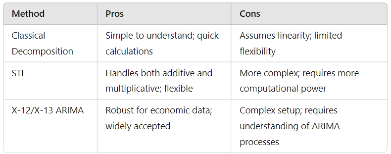
This should give you a clearer picture of which method might be best suited for your needs!
Step-by-Step Example of Time Series Decomposition
Use a Dataset
Now, let’s get practical! I’m going to walk you through a step-by-step example using a well-known dataset: the Airline Passenger Data. This dataset, which tracks the number of airline passengers over time, is a classic in time series analysis.
Imagine you have access to the monthly number of airline passengers from 1949 to 1960. Your goal is to decompose this time series to better understand its trend, seasonality, and noise.
Implementation in Python/R
Here’s how you can implement time series decomposition in Python using the statsmodels library. Let’s say you’ve imported your dataset into a DataFrame named df with a column Passengers.
import pandas as pd
import statsmodels.api as sm
import matplotlib.pyplot as plt

# Load the dataset
df = pd.read_csv('airline_passengers.csv', parse_dates=['Month'], index_col='Month')

# Decompose the time series
decomposition = sm.tsa.seasonal_decompose(df['Passengers'], model='additive')
decomposition.plot()
plt.show()
In this example, I’ve used an additive model for decomposition. The seasonal_decompose function breaks down your series into its components, which we then plot.
If you want to use an R implementation with the forecast package, here’s a snippet for that:
library(forecast)

# Load the dataset
df <- read.csv('airline_passengers.csv')
df$Month <- as.Date(df$Month)

# Decompose the time series
ts_data <- ts(df$Passengers, start=c(1949,1), frequency=12)
decomposition <- decompose(ts_data)
plot(decomposition)
This R code performs similar functions, creating a time series object and decomposing it into trend, seasonal, and random components.
Interpreting the Results
Now that you’ve successfully decomposed your time series, how do you interpret the results?
- Trend Component: Look for the long-term movement in the data. Is it increasing, decreasing, or stable over time? For our airline data, you’ll likely see an upward trend, indicating growing passenger numbers.
- Seasonal Component: Examine the seasonal pattern. In the airline data, you might notice regular peaks during summer months and dips during winter, which is typical for travel patterns.
- Residual (Noise) Component: This is where the randomness lies. You’ll want to check if there are any irregular spikes or dips that can’t be explained by the trend or seasonality. This component helps you identify anomalies or unexpected events.
Conclusion
As we wrap up our journey through the world of time series decomposition, I hope you’ve gained a deeper understanding of this essential technique in data analysis. We’ve explored how time series data, whether it’s airline passenger counts or stock prices, is more than just numbers; it’s a reflection of underlying patterns and trends that can inform decision-making.
Time series decomposition provides you with the tools to dissect these patterns into manageable components: trend, seasonality, and residual noise. By understanding these components, you can uncover insights that would otherwise remain hidden in the complexity of raw data. Whether you opt for classical methods, STL decomposition, or advanced techniques like X-12 ARIMA, you now have a solid foundation to choose the right approach for your data.
Remember, the choice between additive and multiplicative models is crucial, as it can significantly impact your analysis. As you apply these methods to your own datasets, take a moment to reflect on what the results tell you about the world around you.