Q-Learning Algorithms Explained – biased-algorithms.com

Introduction to Reinforcement Learning

Imagine you’re teaching a dog to fetch a ball. You throw the ball, and every time the dog brings it back, you give it a treat. Over time, the dog learns that fetching the ball leads to a reward, so it repeats the behavior. This is the essence of reinforcement learning (RL)—an agent learns to make decisions by interacting with an environment and receiving feedback in the form of rewards.

Context

Reinforcement learning, or RL, is a type of machine learning where agents make a series of decisions by interacting with an environment. The goal? To maximize cumulative rewards. Think of it like a video game—you control a character (the agent), the world of the game is the environment, and every action you take has consequences (positive or negative). The beauty of RL lies in its ability to solve problems without requiring explicit instructions. Instead, the agent learns through trial and error.

Problem Statement

Now, why is RL so crucial? Here’s the deal: RL is the backbone of decision-making systems—whether it’s a robot navigating a room, an AI playing chess, or even self-driving cars avoiding obstacles on the road. The ability to learn from experience makes RL invaluable for tasks where pre-programmed solutions would be insufficient. Traditional rule-based algorithms can’t handle the complexity of dynamic environments the way RL can.

Transition to On-Policy Learning

This might surprise you: Not all RL algorithms learn in the same way. Some algorithms, like Q-Learning, rely on theoretical “best” actions for their updates—what we call “off-policy” learning. But what happens when you want the agent to learn from actual actions it takes? That’s where on-policy learning algorithms like SARSA come in. Instead of learning based on an optimal set of actions, SARSA updates based on the current policy’s actions. It’s like learning on the job—adapting based on what’s happening right now.

What is SARSA?

So, what is this SARSA we’re talking about? Let’s break it down.

Definition

SARSA stands for State-Action-Reward-State-Action. At its core, SARSA is an on-policy reinforcement learning algorithm. In simple terms, this means SARSA learns from the actual actions taken by the agent, not just theoretical best actions.

Acronym Explanation

Here’s how the name SARSA breaks down:

State (S): Where the agent is in the environment.
Action (A): What action the agent chooses to take.
Reward (R): The feedback or reward the agent receives from the environment after taking an action.
Next State (S’): Where the agent ends up after the action.
Next Action (A’): The next action the agent chooses to take in this new state.

Example to Clarify

Let’s say you’re in a maze, and your goal is to find the exit. You start in one corner (your state), and based on your view of the maze, you decide to move forward (your action). If you hit a dead end, the game gives you a negative reward. If you find a clue or get closer to the exit, the game gives you a positive reward. SARSA learns from this entire sequence of states and actions.

On-Policy vs. Off-Policy (SARSA vs. Q-Learning)

You might be wondering, “Why does on-policy matter?” Well, think of Q-Learning like following a map that shows the best route to a destination—even if you’re currently taking a wrong turn, the map doesn’t care about the detours. On the other hand, SARSA is like learning while you drive, adjusting based on the actual streets you’re on. It updates based on the actions you actually take, not just the best possible actions. This makes SARSA particularly useful in situations where exploration could be risky, like controlling a drone or an autonomous vehicle. You don’t want to take the optimal risky move; you want to learn from the safe one you just made.

SARSA Update Rule (Code)

# SARSA Update Formula
# Q(s, a) <- Q(s, a) + α [r + γ Q(s', a') - Q(s, a)]

# Initialize the Q-table with zeros (for simplicity)
Q = np.zeros((number_of_states, number_of_actions))

for each episode:
    state = initial_state
    action = choose_action(state, policy)  # e.g., epsilon-greedy policy

    while not done:
        # Take the action, observe reward and next state
        next_state, reward = environment.step(state, action)
        
        # Choose the next action using the current policy
        next_action = choose_action(next_state, policy)

        # SARSA update rule
        Q[state, action] += alpha * (reward + gamma * Q[next_state, next_action] - Q[state, action])
        
        # Update state and action for the next step
        state = next_state
        action = next_action

Explanation of Code

Initialize the Q-table: We start by initializing the Q-table, which stores the estimated values for each state-action pair.
Episode Loop: For each episode, we start from the initial state and choose an action based on our policy (like ε-greedy).
Action and Reward: After taking an action, we observe the reward and move to the next state.
Choose Next Action: Unlike Q-learning, SARSA immediately selects the next action based on the current policy.
Q-Value Update: We then update the Q-value for the current state-action pair using the SARSA formula. The key difference here is that the update is based on the action we’re actually going to take next, not the best possible action.
Loop Continuation: Finally, we update the state and action for the next step, repeating the process until the episode ends.

How SARSA Algorithm Works: Step-by-Step Explanation

If you’ve ever learned something new—say, how to ride a bike—you probably didn’t master it the first time. You tried, fell, adjusted, tried again, and eventually, you figured out what worked. SARSA works the same way—learning through trial and error, continuously improving its “knowledge” by making decisions, seeing the results, and refining its behavior over time.

Here’s exactly how it works, step by step:

1. Initialization

Before SARSA can start learning, we need to set the stage. In RL terms, this means initializing a Q-value table. This table will store the agent’s knowledge about the environment. Each entry in the table corresponds to a specific state-action pair, and the value in each cell represents the agent’s estimate of how good that action is in that state.

But here’s the twist: initially, the agent has no clue what’s good or bad. So, all the Q-values are usually set to zero (or some small random number), meaning it starts out with no bias toward any specific action.

# Initialize the Q-table to zeros
Q = np.zeros((number_of_states, number_of_actions))

# Alternatively, small random values can be used to encourage exploration.

In this table, every state-action pair will eventually get filled with a number that estimates the expected reward for taking that action in that state. But, we’ll get there soon.

2. Loop Process

Once initialized, SARSA operates in a loop, going through a series of episodes (think of each episode as one complete run from start to finish—like playing a game from beginning to end). Here’s how the loop works:

Step 1: Current State (s)

At any given point, the agent finds itself in a certain state—let’s call it s. For example, in a robot navigation task, the state could represent the robot’s current position in a maze.

Step 2: Choose Action (a)

Now the agent has to make a decision: which action should it take in this state? To do this, it uses a policy. One common approach is the ε-greedy policy, where the agent mostly chooses the action that gives the highest Q-value (exploitation) but occasionally takes a random action (exploration). This helps balance between learning new things and making good decisions based on what it already knows.

action = choose_action(state, Q)  # ε-greedy policy: exploit/explore

Step 3: Take Action and Observe Next State (s’) and Reward (r)

Once the action is chosen, the agent takes that action. As a result, it moves to a new state (s’) and receives a reward (r) based on that action.

For instance, if the robot takes a step closer to its goal, the reward might be positive. If it hits a wall, the reward could be negative.

next_state, reward = environment.step(state, action)  # Move and get feedback

Step 4: Select Next Action (a’) in the New State

Here’s where SARSA’s on-policy nature comes into play. After arriving in the new state (s’), the agent needs to decide its next move. Using the same policy, it chooses another action (a’) in this new state. This is what makes SARSA on-policy—it learns based on the actions it actually takes, not hypothetical best actions.

next_action = choose_action(next_state, Q)  # ε-greedy for next action

Step 5: Update Q-Value Using SARSA’s Formula

This is where the magic happens. SARSA updates its Q-value for the original state-action pair (s, a) using the following formula:

# SARSA Update Rule
Q(s, a) <- Q(s, a) + α [r + γ Q(s', a') - Q(s, a)]

In code form, that looks like this:

# SARSA update
Q[state, action] += alpha * (reward + gamma * Q[next_state, next_action] - Q[state, action])

Let’s break that down:

Q(s, a): This is the current estimate of the value of taking action a in state s.
r: This is the reward the agent received after taking action a in state s.
γ (gamma): This is the discount factor, which determines how much future rewards are valued compared to immediate rewards. Values closer to 1 place more emphasis on future rewards.
Q(s’, a’): This is the estimated value of taking the next action a’ in the new state s’.

The update formula adjusts the Q-value by considering both the immediate reward and the future expected reward. Over time, these updates help the agent form a better understanding of which actions are truly valuable.

Step 6: Update the Current State and Action

After updating the Q-value, the agent prepares for the next step by making the new state (s’) its current state and the next action (a’) its current action.

state = next_state
action = next_action

Termination: When Does the Learning Stop?

You might be wondering: when does the algorithm stop? The learning process continues for a number of episodes, or until the agent has converged—meaning the Q-values no longer change significantly. In practical terms, the algorithm usually runs for a fixed number of episodes or until a performance threshold is reached.

if episode_ends:
    done = True  # The episode ends when a terminal state is reached

3. Graphical Explanation

At this point, it might be helpful to visualize how SARSA works. Imagine a loop where the agent starts in one state, takes an action, moves to the next state, takes another action, and keeps repeating this cycle while updating its Q-values. Over time, these Q-values converge, guiding the agent to make better decisions.

You could create a simple flowchart with the following steps:

Start in state s
Choose action a (based on policy)
Move to next state s’ and get reward r
Choose next action a’ (based on policy)
Update Q-value for state-action pair (s, a)
Repeat until episode ends

This helps solidify the concept in the reader’s mind by showing the cyclical nature of learning through interaction with the environment.

This might seem like a lot to take in, but the beauty of SARSA lies in its simplicity. It’s like learning to ride that bike—every time the agent makes a move, it adjusts based on what works and what doesn’t. Over time, it gets better, making decisions that maximize rewards while minimizing mistakes.

By now, you should have a clear understanding of how SARSA operates, with each step building upon the previous one, ultimately leading the agent to a smarter, more efficient policy.

Mathematical Foundations of SARSA

Let’s face it—math is the backbone of machine learning. When it comes to SARSA, understanding the math helps you truly get why it works. So, let’s unpack it one step at a time.

1. The Bellman Equation: The DNA of SARSA

Here’s the deal: SARSA’s update rule is derived from something fundamental in reinforcement learning—the Bellman equation. This equation tells us how to calculate the expected value of taking an action in a given state by breaking the problem down recursively.

The Bellman equation for Q-values looks like this:

Q(s, a) = r + γ * max(Q(s', a'))

r is the immediate reward the agent receives for taking action a in state s.
γ (gamma) is the discount factor, which we’ll talk about more in a bit.
max(Q(s’, a’)) is the maximum Q-value for the next state s’ and its possible actions.

This is the basis for Q-Learning, where we assume the agent will take the best possible action in the next state.

Now, SARSA modifies this equation slightly because it’s an on-policy algorithm. In SARSA, instead of assuming the agent will take the best action in the next state, it updates based on the action the agent actually takes under the current policy. So, the Bellman equation for SARSA looks like this:

Q(s, a) = r + γ * Q(s', a')

Notice the difference? SARSA updates based on the next action a’ chosen according to the policy (not necessarily the best action). This makes it more realistic when the agent isn’t always acting optimally.

2. SARSA vs. Q-Learning: A Mathematical Comparison

You might be wondering: what’s the real difference between SARSA and Q-Learning? Let’s break it down.

Q-Learning Update Rule

In Q-Learning, the update rule looks like this:

Q(s, a) ← Q(s, a) + α [r + γ * max(Q(s', a')) - Q(s, a)]

What this means is that Q-Learning updates the Q-value for a state-action pair based on the assumption that the agent will take the optimal action in the next state. It always looks ahead and picks the highest possible future reward.

SARSA Update Rule

On the other hand, SARSA’s update rule is:

Q(s, a) ← Q(s, a) + α [r + γ * Q(s', a') - Q(s, a)]

The key difference? SARSA updates based on the actual action a’ that the agent takes in the next state s’, not necessarily the best one. This makes SARSA more conservative in environments where optimal actions may involve risk. It learns from what the agent actually does, not from an idealized best-case scenario.

Why This Makes SARSA On-Policy

The reason SARSA is called on-policy is simple: it updates based on the current policy the agent is following. The action taken in the next state is determined by the agent’s policy, not by always choosing the action with the highest Q-value. This is particularly useful when you want the agent to learn while following a specific strategy—like balancing exploration and exploitation.

Think of it this way: Q-Learning is like assuming you’ll always make the best choice in the future, while SARSA is like learning from the choices you actually make. It’s like life—sometimes you don’t know the best path, so you learn as you go.

3. Discount Factor (γ) and Learning Rate (α)

Now, let’s talk about the two magic knobs you can turn to control how SARSA learns: the discount factor (γ) and the learning rate (α). These hyperparameters play a massive role in determining the quality and speed of learning.

Discount Factor (γ)

The discount factor (γ) controls how much weight the agent places on future rewards versus immediate rewards. In other words, γ determines how much the agent “cares” about long-term gains compared to short-term benefits.

If γ = 0, the agent is totally short-sighted, only focusing on immediate rewards. It won’t care about the future at all.
If γ = 1, the agent values future rewards just as much as immediate rewards, making it extremely patient.

You might be wondering, “What’s the right value for γ?” Well, it depends on your problem. In environments where long-term planning is important (like chess or autonomous driving), a higher γ is usually better. In situations where immediate rewards are critical (like stock trading), a lower γ might work better.

Learning Rate (α)

The learning rate (α) is another key parameter that controls how quickly the agent updates its Q-values after each action. It determines how much new information overrides old knowledge.

If α = 0, the agent never learns anything new, sticking to its initial estimates.
If α = 1, the agent immediately overwrites old information with new information after each action.

The trick is finding the sweet spot for α. If α is too high, the agent may overreact to new information and never stabilize. If α is too low, the agent learns too slowly, making little progress in refining its strategy.

In practice, values of α are usually kept small (e.g., 0.1 to 0.5) to allow gradual learning over time.

Final Thoughts:

In a nutshell, SARSA is like an agent learning on the job—updating its knowledge based on what’s actually happening, not on theoretical best actions. By adjusting the discount factor (γ) and learning rate (α), you control how focused the agent is on immediate rewards vs. long-term rewards and how fast it learns from its experiences.

Practical Example with Code (Python Implementation)

Alright, so let’s see SARSA in action. To truly grasp how SARSA learns, it’s important to move from theory into practice. In this example, we’ll use OpenAI Gym’s CliffWalking-v0 environment—a perfect setting to demonstrate SARSA because it’s a gridworld where poor decisions lead to a steep “fall” off a cliff (negative rewards), and careful, calculated steps lead to success (positive rewards).

Environment Setup: OpenAI Gym’s “CliffWalking-v0”

Before we get started, you’ll need to install OpenAI Gym if you haven’t already. You can install it via pip:

pip install gym

In this environment:

You control an agent that navigates a 4×12 grid from the start (top-left corner) to the goal (bottom-right corner).
There’s a cliff along the bottom edge. If the agent falls off, it receives a high negative reward (-100) and returns to the start.
The goal is to maximize rewards while avoiding the cliff and reaching the goal.

SARSA Code: Step-by-Step Implementation

Now, let’s dive into the code.

import gym
import numpy as np

# Create the environment
env = gym.make('CliffWalking-v0')

# Initialize parameters
alpha = 0.1   # Learning rate
gamma = 0.99  # Discount factor
epsilon = 0.1  # Epsilon for ε-greedy policy
num_episodes = 500  # Number of episodes to train

# Initialize Q-table with zeros (number of states x number of actions)
Q = np.zeros((env.observation_space.n, env.action_space.n))

# Function to choose action using ε-greedy policy
def choose_action(state, Q, epsilon):
    if np.random.rand() < epsilon:
        # Explore: choose a random action
        return env.action_space.sample()
    else:
        # Exploit: choose the action with the highest Q-value for this state
        return np.argmax(Q[state, :])

# Training loop
for episode in range(num_episodes):
    state = env.reset()  # Reset the environment at the start of each episode
    action = choose_action(state, Q, epsilon)  # Choose an initial action using ε-greedy policy

    done = False
    while not done:
        next_state, reward, done, info = env.step(action)  # Take the action and observe the outcome
        next_action = choose_action(next_state, Q, epsilon)  # Choose the next action using ε-greedy

        # SARSA update rule
        Q[state, action] += alpha * (reward + gamma * Q[next_state, next_action] - Q[state, action])

        # Move to the next state and action
        state = next_state
        action = next_action

# Show learned Q-values
print("Learned Q-values:")
print(Q)

# Test the agent
state = env.reset()
done = False
while not done:
    action = np.argmax(Q[state, :])  # Choose the best action from the learned Q-table
    next_state, reward, done, info = env.step(action)
    env.render()  # Visualize the agent's movement
    state = next_state

env.close()

Comparison Between SARSA and Other RL Algorithms

Reinforcement learning is a vast field, with multiple algorithms tailored for different scenarios. So, how does SARSA measure up against some of the other popular algorithms out there? Let’s break it down.

1. SARSA vs. Q-Learning: A Head-to-Head Comparison

Here’s the deal: both SARSA and Q-Learning are trying to solve the same problem—how to learn the best way to behave in an environment. But they do it in slightly different ways.

Policy Type

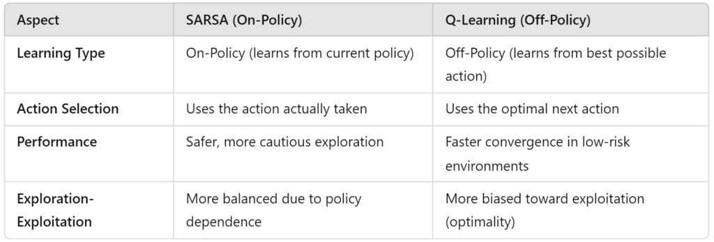
SARSA is an on-policy algorithm. This means it learns from the actions it actually takes while following a specific policy. The updates it makes are based on the current action selection strategy, balancing exploration and exploitation.
Q-Learning, on the other hand, is off-policy. It learns from the best possible actions, regardless of whether the agent is actually taking those actions. It assumes the agent will always act optimally, even if it doesn’t in practice.

Action Selection

SARSA updates its Q-values based on the action the agent actually took, which means it considers how the policy behaves in the real world. For example, if you have an exploratory policy (like ε-greedy), SARSA updates based on that exploration.
Q-Learning updates the Q-values using the best possible action in the next state, even if the agent doesn’t take that action. It’s like betting on the optimal outcome, assuming the agent knows exactly what to do next (even if it’s still exploring).

Performance in Different Environments

SARSA is often better suited for safer exploration. Since it updates based on the current policy (which may explore), it tends to be more cautious. In high-risk environments (like our earlier example of navigating a cliff), SARSA is the safer choice because it learns from the actions that were actually taken, not the best-case scenario.
Q-Learning shines in environments where maximizing long-term rewards is the goal and where it’s okay to assume the agent will always act optimally. It’s faster in environments with low risk because it immediately optimizes for the best possible actions, even if those actions weren’t the ones taken.

Here’s a quick comparison for clarity:

2. SARSA vs. Deep Q-Networks (DQN): A Look into the Future of RL

You might be wondering, “What about more advanced algorithms, like Deep Q-Networks (DQN)?” Well, here’s where things get even more interesting.

DQN extends Q-Learning by using neural networks to approximate the Q-values for very large state spaces. Instead of relying on a Q-table, which becomes impractical for complex environments, DQN uses a deep neural network to predict the Q-values for each action.

How SARSA Compares to DQN:

SARSA is great for small, discrete state spaces where a simple table of Q-values is manageable. It’s easy to implement, understand, and interpret.
DQN, however, is designed for high-dimensional, continuous environments like video games (think Atari, where DQN was first used). When the number of states becomes too large to handle with a table, DQN steps in and uses the power of deep learning to generalize across these states.

Where SARSA Still Shines:

Simplicity and Transparency: SARSA is easy to debug and tune. Its updates are straightforward, making it ideal for smaller problems where interpretability matters.
Safe Exploration: In environments where exploration carries a significant risk (like autonomous driving or robotics), SARSA’s on-policy nature makes it more conservative and potentially safer than DQN or other off-policy algorithms.

So, while SARSA may not be as powerful as DQN for large-scale problems, it’s still highly effective when you need control over the exploration process and a simpler, more interpretable approach.

3. When to Use SARSA

Now, let’s talk about when SARSA might be the best tool for the job. Here are a few scenarios where SARSA tends to outperform other algorithms:

Risky Environments: When exploring new actions carries a risk of significant penalties (like falling off a cliff or damaging equipment), SARSA’s conservative, on-policy learning can help the agent avoid dangerous actions more effectively than Q-Learning or DQN.
Smaller, Discrete State Spaces: If your problem can be solved with a Q-table (where the number of states is manageable), SARSA is an excellent choice. It’s simple to implement, easy to interpret, and requires fewer computational resources than more complex methods like DQN.
When You Need Safer Exploration: In real-world systems, such as healthcare, finance, or robotics, where exploration might lead to costly mistakes, SARSA’s ability to learn from the current policy’s actions can make it more practical than Q-Learning, which assumes optimal actions even during exploration.

Conclusion

So, what’s the takeaway here?

SARSA offers a practical, reliable approach to reinforcement learning, particularly when you need safer exploration and are working within smaller or more discrete environments. It may not have the raw power of more advanced techniques like Deep Q-Networks, but its ability to balance exploration and exploitation in risky environments gives it a unique edge.

Whether you’re building autonomous systems, experimenting with small gridworld environments, or just want to dive into reinforcement learning with a simpler algorithm, SARSA is a solid choice. By understanding the core principles of SARSA—and how it compares to other RL methods—you’ll be better equipped to choose the right algorithm for your specific problem.

In the world of RL, no single algorithm fits all problems. But when safety, simplicity, and policy-driven learning matter, SARSA is your go-to.