
Have you ever looked at a giant spreadsheet filled with mostly empty cells and thought, “There’s got to be a more efficient way to store this”? Well, that’s where sparse datasets come into play.
A sparse dataset is essentially a dataset where most of the values are either zero or empty. Think of it like a concert hall where only a few seats are occupied and the rest are empty — the people are the actual data points, and the empty seats are the zeros. Sparse data can be found across various domains and is crucial for working efficiently with modern machine learning algorithms and large datasets.
Why It Matters:
Here’s the deal: Data in the real world often comes with a lot of missing or irrelevant values. For example, let’s say you’re working on a recommendation system where you have thousands of users and millions of products, but most users will only interact with a tiny fraction of those products. This leads to a sparse dataset, with most entries being zeros (no interaction).
Sparse datasets are everywhere! From text data (where documents contain only a few words from an extensive vocabulary) to user-item recommendation systems and even bioinformatics (with gene expression data where only certain genes are active), sparsity is something you’ll face more often than you think.
Common Domains:
Let’s break it down. You’ll most frequently encounter sparse datasets in the following areas:
- Text Data: When processing large text corpora, tools like TF-IDF (Term Frequency-Inverse Document Frequency) convert words into vectors. A text document usually has a few relevant words, with the rest of the dictionary being unused, making the resulting vectors sparse.
- Recommendation Systems: Picture Netflix or Amazon, where users rate only a fraction of all available movies or products. These user-item interaction matrices are highly sparse because most users interact with only a small percentage of the items.
- Bioinformatics: Gene expression data can also be sparse because not all genes are expressed in all conditions, leading to many zeros in the dataset.
By now, you’re probably seeing the pattern: wherever you have large datasets and relatively few meaningful entries, you’re likely dealing with sparsity. Understanding how to handle these efficiently can give you a big edge in optimizing storage and computation.
Dense vs. Sparse Datasets
Before we get too deep into sparse datasets, it’s essential to compare them with their counterpart: dense datasets. Imagine dense data as a tightly packed suitcase — everything has a place, and there’s little to no empty space. Dense datasets have meaningful values in most of their elements. A classic example is an image dataset where every pixel in an image has a value, and there are few or no empty entries.
Key Differences:
Here’s a quick table to help you visualize the differences between dense and sparse datasets:
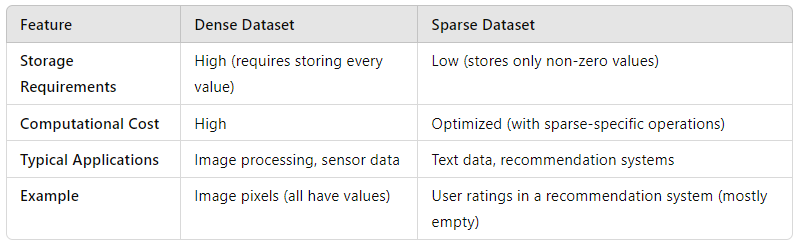
Impact on Algorithms:
Now, let’s talk about how this impacts the algorithms you’re using. Machine learning algorithms are typically designed to handle dense datasets. However, when faced with sparse data, some algorithms may struggle. Why? Because they aren’t optimized to ignore those zero or empty values. For instance, a basic matrix multiplication in dense form can be computationally expensive because it processes every entry, including the zeros.
In contrast, algorithms that are designed to handle sparsity, like logistic regression with L1 regularization, shine in these scenarios. They know how to ignore zeros efficiently, speeding up computation and reducing memory usage. Specialized libraries, like scipy.sparse in Python, take advantage of this by storing and processing only the non-zero elements of a matrix, saving both time and resources.
Characteristics of Sparse Datasets
Let’s talk about a strange, but fascinating phenomenon in the world of data: high-dimensional spaces that are mostly…empty. You might think, “Why would we need a dataset with so many dimensions if most of them are zeros?” Well, welcome to the nature of sparse datasets!
High-Dimensional Data:
Sparse datasets often come with a large number of dimensions, or features, but only a small fraction of these dimensions have actual values. For example, if you’re working with a dataset where each feature represents a word in a text document, imagine how many potential words there could be! A document might only use a tiny percentage of them, leaving the rest as zeros.
To put this in perspective: If you had a matrix of 1,000,000 words and 100,000 documents, but each document only uses about 100 words, the rest of the matrix will be zeroes. That’s what makes sparse datasets so intriguing and also so challenging. They are like enormous galaxies where most of the stars (data points) are missing, and only a few shine.
Zeros in the Dataset:
Now, you might be wondering: Why all the zeros? This is called zero inflation, and it’s not a bug — it’s a feature. Sparse datasets are typically filled with zeros because many of the potential interactions or relationships simply don’t exist. Think of a user-rating system where not every user rates every product. Most users won’t touch most products, so the data matrix is mostly zeros.
In bioinformatics, for example, genes are expressed only under specific conditions, meaning that in many contexts, they remain inactive, leaving large portions of your data filled with zeros. But here’s the thing: Those zeros matter. They tell you where interactions didn’t happen or where features were not present, giving you clues about the structure of your data.
Memory and Computational Considerations:
Here’s where things get practical: If you were to store all those zeros in memory, you’d run out of space quickly, not to mention your computations would crawl. That’s why we handle sparse data differently. Sparse matrices are stored in specialized formats like Compressed Sparse Row (CSR) or Compressed Sparse Column (CSC), which only store the non-zero elements, along with their positions. This means you can work with large datasets more efficiently, using much less memory and faster computations.
If you’ve ever tried matrix multiplication with a dense matrix versus a sparse matrix, you’ll know that the difference in speed is night and day. By storing only the meaningful values, your algorithm can zip through the matrix, ignoring those zeros, making computations lightning fast.
Practical Examples of Sparse Datasets
Now, let’s dive into some real-world examples where sparse datasets are not just common, but essential. These examples will help you connect the theory to practical use cases.
Text Data:
Imagine you’re building a natural language processing (NLP) model. You’ve got thousands of documents, each filled with words from an enormous vocabulary. But here’s the catch: most documents only use a small subset of those words, leaving the rest of the word-space blank. This creates a sparse dataset.
Take, for instance, the TF-IDF (Term Frequency-Inverse Document Frequency) representation of text. It’s a way to transform text into numerical vectors, but it often results in sparse matrices because each document only contains a few significant words. Here’s a quick example in Python to illustrate this:
from sklearn.feature_extraction.text import TfidfVectorizer

documents = ["Sparse datasets are common in NLP",
             "Machine learning can handle sparse matrices",
             "TF-IDF helps represent sparse text data"]

vectorizer = TfidfVectorizer()
X = vectorizer.fit_transform(documents)
print(X)  # This will output a sparse matrix
In this example, even though there are hundreds of potential words, each document only uses a fraction, leading to a sparse matrix. If you were to visualize this matrix, it would be mostly zeros, with just a few non-zero entries representing the important words.
Recommendation Systems:
This might surprise you, but most recommendation systems — think Netflix or Amazon — are driven by sparse data. Here’s why: out of the thousands of movies available, most users will only rate a handful. So, when you build a user-item interaction matrix, most of the cells in the matrix will be empty or zero, representing items that haven’t been rated.
Let’s consider an example:
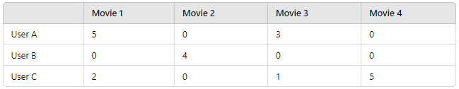
Here, you can see that users only rate a few movies. This creates a sparse matrix where most of the values are zeros, indicating no interaction between users and certain movies.
Bioinformatics:
In the world of bioinformatics, sparse data is everywhere. Let’s say you’re studying gene expression. Not all genes are expressed in every condition or tissue, so the resulting dataset, which tracks which genes are “active,” ends up being mostly zeros. For instance, a matrix representing gene expression might look something like this:
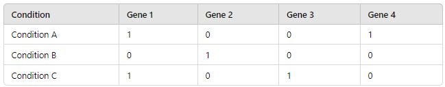
Here, a “1” represents a gene that’s expressed, while a “0” indicates no expression. You can see how sparse this matrix is — most genes aren’t active in each condition.
Computer Vision:
Now, you might not think of computer vision as a domain that deals with sparse data, but there’s a twist: pixel activation matrices in certain image processing tasks can be sparse. For instance, in object detection, not every pixel in an image is activated to represent an object. Only the pixels where the object appears have non-zero values, leading to a sparse matrix of activations.
Let’s say you’re analyzing an image with a sparse activation map:
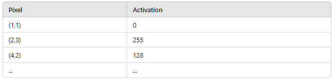
Only a few pixels are activated, and the rest remain zero. This sparsity can significantly reduce the computational cost, especially in large-scale image datasets.
Storing Sparse Data
Here’s the thing: when it comes to storing sparse data, traditional data structures are like trying to store air in a suitcase — inefficient and impractical. You wouldn’t want to waste space storing all those zeros in memory, would you?
Challenges with Storing Sparse Data:
Let me paint you a picture. Suppose you’re working with a large matrix — let’s say 1,000,000 rows by 1,000 columns — but 99% of the values in this matrix are zeros. If you try to store it as-is, you’d waste a huge amount of memory on storing all those zeros, leaving your system choked with unnecessary data.
What’s worse is that many operations, like matrix multiplication or addition, would end up being incredibly slow because every zero needs to be processed. And let’s face it: your algorithm doesn’t need those zeros; they add nothing to the computation.
This brings us to the crux of the problem: how do you store only the meaningful values (non-zero values) and ignore the rest?
Efficient Storage Formats:
Luckily, data science has a few tricks up its sleeve. There are specialized formats designed to store sparse data efficiently, and they only keep track of the non-zero values. Here are three common formats you’ll often use:
- COO (Coordinate Format): Think of this as the simplest approach. The COO format stores the coordinates of non-zero elements along with their values. It’s easy to construct but not the most efficient for computations.
- CSR (Compressed Sparse Row): Now we’re talking optimization. In the CSR format, we store the non-zero values row by row, compressing the data by keeping track of where each row starts and ends. This format is much faster for row-based operations, like matrix-vector multiplication.
- CSC (Compressed Sparse Column): If your operations are column-based, CSC is your go-to. This format is similar to CSR but compresses the data column by column instead of row by row.
You might be wondering: “Which one should I use?” Well, it depends on the operations you’re performing. If you’re doing a lot of row-based operations (like dot products), go with CSR. If you’re working with columns, CSC might be a better choice.
Example in Python:
Here’s a quick Python snippet to show how you can store a sparse matrix using the scipy.sparse library. Let’s say we’ve got a simple matrix:
import numpy as np
from scipy.sparse import coo_matrix, csr_matrix, csc_matrix

# Define a simple 5x5 matrix
data = np.array([3, 4, 5])
rows = np.array([0, 1, 3])
cols = np.array([0, 2, 4])

# Create a COO sparse matrix
coo = coo_matrix((data, (rows, cols)), shape=(5, 5))
print("COO format:\n", coo)

# Convert to CSR format
csr = coo.tocsr()
print("\nCSR format:\n", csr)

# Convert to CSC format
csc = coo.tocsc()
print("\nCSC format:\n", csc)
In this example, you can see how we store only the non-zero values and use different formats to make the storage and computation more efficient.
Working with Sparse Data in Python
Now that we’ve figured out how to store sparse data, let’s move on to the real fun: working with it. Python has some fantastic tools that let you manipulate sparse data with ease.
Sparse Matrix Representation:
In Python, the two most commonly used libraries for dealing with sparse data are scipy and sklearn. Whether you’re working on building a machine learning model or simply trying to manipulate large datasets, these libraries offer efficient ways to represent sparse matrices without storing all the zeros.
For example, let’s create a CSR matrix in Python using scipy.sparse:
from scipy.sparse import csr_matrix

# Create a dense matrix (just for illustration)
dense_matrix = np.array([[0, 0, 1], [1, 0, 0], [0, 2, 0]])

# Convert to a sparse matrix
sparse_matrix = csr_matrix(dense_matrix)

print("Sparse Matrix (CSR):\n", sparse_matrix)
In the above example, you start with a dense matrix but quickly transform it into a sparse representation, saving memory space in the process. And the best part? Your computations will run faster with this optimized representation.
Operations on Sparse Matrices:
Once you have your sparse matrix, what next? Well, you can perform a variety of operations on it — like addition, multiplication, or dot products — but these work differently from dense matrix operations.
Let me give you a practical example. Let’s say you want to multiply two sparse matrices. With dense matrices, each zero value would still be included in the multiplication. But in sparse matrices, only the non-zero values are considered, speeding up the process considerably.
# Create two sparse matrices
sparse_matrix_1 = csr_matrix([[0, 0, 3], [1, 0, 0], [0, 2, 0]])
sparse_matrix_2 = csr_matrix([[0, 1, 0], [2, 0, 0], [0, 0, 4]])

# Perform matrix multiplication
result = sparse_matrix_1.dot(sparse_matrix_2)

print("Result of multiplication:\n", result)
Here, instead of wasting resources multiplying zeros, we focus on the non-zero values. In this example, sparse_matrix_1 and sparse_matrix_2 are multiplied together in an efficient manner.
You can also perform element-wise operations. For instance, adding two sparse matrices is as simple as adding their non-zero values. The zeros stay zeros, and only the actual data points are modified:
# Perform element-wise addition
sum_matrix = sparse_matrix_1 + sparse_matrix_2

print("Result of addition:\n", sum_matrix)
As you can see, operations with sparse matrices are not only faster but also memory-efficient. You won’t waste time or space on unnecessary values, which makes these techniques critical when you’re working with large-scale data.
Machine Learning with Sparse Datasets
Alright, here’s where things get really interesting. When it comes to machine learning with sparse datasets, you’re probably thinking: “Do traditional algorithms even work with all those zeros?” The short answer is yes — but not all algorithms are created equal. Some models are tailor-made to handle sparse inputs more efficiently, while others struggle and require specific adaptations.
Handling Sparsity in ML Models:
First, let’s talk about why sparsity matters in machine learning. Imagine you’re working with a dataset where 90% of the data points are zeros. Standard algorithms treat every data point equally, meaning they waste time and computational power processing all those zeros. This leads to inefficiencies, and in some cases, even poor performance.
But here’s the deal: certain algorithms are naturally better equipped to deal with sparse datasets. These models can focus only on the non-zero values, speeding up training times and improving accuracy. So, let’s look at a few of these algorithms that work well with sparse data.
Algorithms Suited for Sparse Data:
- Logistic Regression (with regularization):When working with sparse datasets, logistic regression can be a surprisingly effective choice, especially when regularized. L1 regularization (Lasso) helps by penalizing non-zero coefficients, which is ideal for sparse data. It essentially acts as a feature selector, driving less important features toward zero.Example in Python:
from sklearn.linear_model import LogisticRegression
from scipy.sparse import csr_matrix
import numpy as np

# Create a sparse dataset
X = csr_matrix([[0, 1, 0], [0, 0, 1], [1, 0, 0], [0, 1, 1]])
y = np.array([0, 1, 0, 1])

# Logistic regression with L1 regularization (Lasso)
model = LogisticRegression(penalty='l1', solver='liblinear')
model.fit(X, y)

print("Model coefficients:", model.coef_)
- In this example, L1 regularization forces some of the coefficients to zero, which is especially useful in sparse datasets with high dimensions. This way, the model learns only the relevant features.
- SVM (Support Vector Machines) with a Sparse Kernel:Support Vector Machines (SVM) can also handle sparse datasets, but there’s a catch: you need to use sparse kernels. These kernels are specifically designed to handle sparse inputs, ensuring that SVM focuses only on the non-zero entries. SVMs are great for high-dimensional sparse datasets like text classification tasks.Example in Python:
from sklearn.svm import SVC

# SVM on a sparse dataset
svm_model = SVC(kernel='linear')
svm_model.fit(X, y)

print("SVM support vectors:", svm_model.support_vectors_)
- In this case, the
linearkernel efficiently handles the sparse input matrix, allowing SVM to find the optimal hyperplane without wasting resources on the zeros.
- Decision Trees and Random Forests:Decision trees and Random Forests are another solid choice when working with sparse data. Why? Because they split features at decision nodes, and if a feature doesn’t contribute (like a column full of zeros), the algorithm can effectively ignore it. This makes them naturally robust to sparsity.Example in Python:
from sklearn.ensemble import RandomForestClassifier

# Random Forest on sparse data
rf_model = RandomForestClassifier()
rf_model.fit(X, y)

print("Feature importances:", rf_model.feature_importances_)- In this case, the random forest model will automatically ignore features that provide no information (i.e., the all-zero columns), making it ideal for sparse datasets.
Deep Learning with Sparse Data:
Now, let’s take it up a notch. Deep learning might seem like a bad fit for sparse datasets, but here’s the surprising part: it can work exceptionally well if you use the right techniques.
One effective approach is to use sparse autoencoders. These neural networks are designed to learn a compressed representation of your data while maintaining the important features, ignoring the zeros. They’re particularly useful for dimensionality reduction and learning efficient encodings for high-dimensional sparse data.
Example: Sparse Neural Network in PyTorch
Let’s walk through a simple sparse neural network using PyTorch. We’ll create a sparse input and train an autoencoder to compress and reconstruct it.
import torch
import torch.nn as nn
import torch.optim as optim

# Define a simple sparse autoencoder
class SparseAutoencoder(nn.Module):
    def __init__(self, input_size, hidden_size):
        super(SparseAutoencoder, self).__init__()
        self.encoder = nn.Linear(input_size, hidden_size)
        self.decoder = nn.Linear(hidden_size, input_size)

    def forward(self, x):
        encoded = torch.relu(self.encoder(x))
        decoded = torch.sigmoid(self.decoder(encoded))
        return decoded

# Create a sparse dataset
X = torch.tensor([[0, 1, 0], [0, 0, 1], [1, 0, 0], [0, 1, 1]], dtype=torch.float32)

# Model and optimizer
input_size = X.shape[1]
hidden_size = 2
model = SparseAutoencoder(input_size, hidden_size)
optimizer = optim.Adam(model.parameters(), lr=0.01)
criterion = nn.MSELoss()

# Train the autoencoder
for epoch in range(100):
    output = model(X)
    loss = criterion(output, X)
    optimizer.zero_grad()
    loss.backward()
    optimizer.step()

print("Reconstructed output:\n", output)
In this example, the autoencoder learns a compressed version of the sparse input data. After training, it tries to reconstruct the original data from this compressed representation, ignoring the unnecessary zeros.
Conclusion
Congratulations! You’ve made it to the end of this deep dive into the world of sparse datasets. Let’s quickly recap the key takeaways:
Sparse datasets are not only common but crucial in many fields like text processing, recommendation systems, and bioinformatics. Understanding how to efficiently store, manipulate, and build machine learning models on these datasets can make a huge difference in both performance and accuracy. From specialized storage formats like COO, CSR, and CSC to choosing the right machine learning algorithms (like logistic regression with L1 regularization, SVM with sparse kernels, or random forests), sparsity is a challenge you can overcome — and even use to your advantage.
Whether you’re dealing with millions of rows in a recommendation system or high-dimensional gene expression data, mastering sparsity will save you memory, computation time, and — most importantly — help you make smarter, faster decisions with your data.
Now, it’s your turn. Take these concepts and examples, experiment with them in your own projects, and see the power of sparse data in action. Sparse data is more than just a technical quirk — it’s a tool to enhance your machine learning workflows.
And remember: less is more when it comes to sparsity!