
1. Introduction to Bag of Words (BoW)
“You can’t manage what you can’t measure.” This famous quote applies to many fields, including Natural Language Processing (NLP). When you’re dealing with text, one of the most crucial tasks is to measure words in a meaningful way, and that’s where the Bag of Words (BoW) model comes into play.
Definition
So, what exactly is Bag of Words? At its core, it’s a technique that represents text data in a simplified form, reducing it to a set of word frequencies. Imagine you have a sentence like, “The quick brown fox jumps over the lazy dog.” With BoW, the model doesn’t care about grammar, word order, or the deeper meaning of the sentence. It simply breaks down the sentence into individual words and counts how often each word appears.
Here’s the deal: BoW converts text into numerical data by creating a “bag” of words from your dataset. Every unique word gets its own position, and your text becomes a vector that represents the frequency of those words. Sounds simple, right? Well, that’s the beauty of it—BoW is all about simplicity.
Importance in NLP
Now, you might be wondering, why is such a basic technique still so fundamental in NLP? Because text data is messy and unstructured. BoW provides a structured way to handle this mess. It’s a reliable first step to transform raw text into something a machine can understand. Tasks like text classification (categorizing emails into spam or not spam), sentiment analysis (identifying positive or negative emotions), and even document clustering often use BoW as a starting point.
In fact, if you’ve ever worked with machine learning models involving text, chances are you’ve already encountered BoW. It’s like the backbone of many text-based models, providing the essential framework for algorithms to process natural language.
Applications
You’ll find BoW used in countless applications. It’s popular in machine learning models for:
- Text classification: Think spam filters or categorizing product reviews.
- Document similarity analysis: Matching documents or web pages based on word overlap.
- Topic modeling: Grouping texts by topics based on word distribution.
BoW’s simplicity makes it versatile. Whether you’re analyzing Twitter sentiment or training a chatbot, this technique helps in breaking down text data in a straightforward way.
BoW vs. Other Methods
But here’s where it gets interesting: Bag of Words is not the only game in town. You’ve got other methods like TF-IDF (Term Frequency-Inverse Document Frequency) and Word Embeddings (such as Word2Vec or BERT). While BoW focuses on raw word counts, TF-IDF assigns more importance to rare words that carry more meaning. On the other hand, Word Embeddings aim to capture context and semantic meaning, going far beyond the simplicity of BoW.
So, when is BoW more appropriate? If you’re working on a project where simplicity and interpretability matter more than understanding deep context—such as early-stage text mining or fast prototyping—BoW is your best friend. It’s quick, easy, and effective for tasks where context isn’t critical.
2. How Bag of Words Works
Let’s break down the mechanics of Bag of Words. If you’re familiar with cooking, think of this as your recipe for preparing raw text into something a machine can consume.
Tokenization
First, you need to chop the text up. This process is called tokenization, where your text is broken down into individual words or “tokens.” For instance, the sentence “I love NLP” would be tokenized into ["I", "love", "NLP"]. At this stage, your goal is to treat each word as a separate unit of meaning.
Text Normalization
Next, it’s time to clean up. Text data can be messy—uppercase letters, punctuation, numbers, and stopwords (common words like “and,” “the,” or “in” that don’t add much meaning). During text normalization, you’ll:
- Convert everything to lowercase to avoid treating “Cat” and “cat” as different words.
- Remove punctuation and numbers.
- Eliminate stopwords to reduce noise in the data.
Now, imagine you’re working with a product review: “This product is AMAZING! I would buy it again 100 times.” After normalization, it might look something like this: ["product", "amazing", "buy", "times"]. You’ve kept only the essential words.
Creating a Vocabulary
Here’s where things get structured. After you’ve tokenized and cleaned your text, you build a vocabulary—a list of all unique words in your dataset. Think of it as creating a dictionary where every word in your dataset gets a specific index.
If you’re working with a larger text corpus, the vocabulary can be massive. For instance, if you’re analyzing hundreds of customer reviews, your vocabulary might consist of thousands of words.
Vectorization
Next up is vectorization, where the magic happens. Here’s how it works: each document in your dataset is transformed into a fixed-size vector. Each position in the vector corresponds to a word in your vocabulary, and the value in that position represents how many times that word appears in the document.
For example, if your vocabulary is ["amazing", "buy", "product", "times"] and your document is “This product is amazing,” the corresponding vector might look like [1, 0, 1, 0], because “amazing” and “product” each appear once, while “buy” and “times” do not appear.
Term Frequency Calculation
You might be thinking, how exactly are these values calculated? It’s all about term frequency (TF)—the number of times a word appears in a document. The higher the frequency, the higher the importance of that word within the document. But keep in mind, the term frequency only reflects a word’s importance within a single document, not across all documents.
Dimensionality Issues
Now, let’s address a challenge you’ll likely face: dimensionality. When you have a huge vocabulary and many documents, your vectors can become extremely large, leading to high-dimensionality. This can slow down your machine learning models and make them harder to interpret.
A simple solution? You can reduce dimensionality by filtering out rare or unimportant words, or using techniques like dimensionality reduction (such as PCA) to keep only the most informative features.
3. Implementing Bag of Words in R
As the saying goes, “Practice makes perfect.” So, it’s time to roll up your sleeves and implement Bag of Words (BoW) in R! I’m sure you’ve already seen how useful BoW can be conceptually, but now let’s walk through the practical steps. This section will help you understand how to take raw text data and transform it into something your machine learning model can digest.
Required Libraries
Before you jump in, you’ll need the right tools. R has some fantastic packages that make text mining a breeze:
tm: This is your go-to package for basic text mining tasks, especially when creating Document-Term Matrices (DTM).quanteda: If you’re looking for something more powerful,quantedaexcels in quantitative text analysis and handling larger datasets.tidytext: As the name suggests, this package aligns text mining with the tidy data principles, making it easier to integrate with tools likedplyrandggplot2.
Here’s the deal: Depending on your project size and goals, you can choose the package that best fits your workflow. For now, let’s work with tm to keep things simple.
Example Dataset
To give you something concrete, let’s say you’re working with a dataset of product reviews. These reviews can be as simple as a few sentences or paragraphs describing the user’s experience. For this walkthrough, imagine a small dataset where customers talk about their favorite gadgets.
a) Step-by-Step Code Walkthrough
Step 1: Loading the Dataset First things first—you’ve got to load your text data into R. Let’s assume your data is stored in a plain text format or CSV.
# Loading the necessary libraries
library(tm)

# Assuming 'text_data' contains a vector of customer reviews
docs <- Corpus(VectorSource(text_data))
In this case, Corpus is like the container that holds your collection of documents (your reviews, for example). You’ll feed your raw text into this structure.
Step 2: Text Preprocessing Here’s where you clean up the mess! Real-world text data is far from perfect. Punctuation, numbers, and irrelevant words are your enemies here, and you need to get rid of them to make the data machine-friendly.
# Converting to lowercase
docs <- tm_map(docs, content_transformer(tolower))

# Removing punctuation
docs <- tm_map(docs, removePunctuation)

# Removing numbers
docs <- tm_map(docs, removeNumbers)

# Removing stopwords (common words like "the", "and", etc.)
docs <- tm_map(docs, removeWords, stopwords("en"))
You might be wondering, why go through all this hassle? Well, machines are quite literal. If you don’t normalize the text, “Amazing” and “amazing” will be treated as different words, and punctuation will throw your models off.
Optional: Stemming or Lemmatization If you want to take things further, you can perform stemming (reducing words to their root form) or lemmatization (similar to stemming but more context-aware). For instance, “running” and “runs” could be reduced to “run” for more compact features.
# Stemming (optional)
library(SnowballC)
docs <- tm_map(docs, stemDocument)
Step 3: Creating a Document-Term Matrix (DTM) Now that your text is clean, it’s time to create the Document-Term Matrix (DTM). A DTM is where each row represents a document, and each column represents a word from your vocabulary. The cells contain word counts.
# Creating the Document-Term Matrix
dtm <- DocumentTermMatrix(docs)

# Inspect the matrix
inspect(dtm)
At this point, you’ve transformed your text data into a structured format. Your dataset might now look something like this:
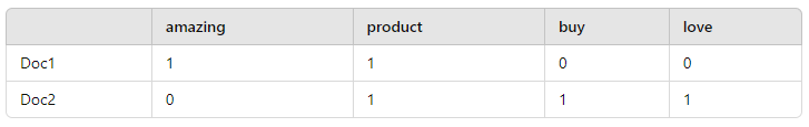
Each document is now represented as a numerical vector based on word frequency.
Step 4: Sparse Matrix You might have noticed that most of the matrix cells are filled with zeros. That’s because most words don’t appear in every document—this leads to a sparse matrix. While a sparse matrix is great for saving memory, it can pose computational challenges, especially with large vocabularies. R has packages like Matrix and slam to handle these efficiently.
# Convert the DTM into a sparse matrix for better efficiency
library(Matrix)
sparse_dtm <- as(dtm, "sparseMatrix")
That’s it! You’ve successfully implemented Bag of Words in R. Now your text data is ready for machine learning models or further analysis.
4. Advanced Concepts in Bag of Words
You’ve mastered the basics, but you’re probably thinking, What’s next? BoW is just the starting point. Let’s explore some advanced concepts that can enhance your text analysis.
Term Frequency-Inverse Document Frequency (TF-IDF)
This might surprise you, but not all words are created equal. Common words like “product” or “buy” might appear frequently across many documents, but they don’t provide much insight. TF-IDF is a method that not only counts word frequency (like BoW) but also penalizes common words by weighing them less.
Here’s how it works: The Term Frequency (TF) represents how often a word appears in a document, while the Inverse Document Frequency (IDF) measures how rare a word is across the entire dataset. The result? Words that are frequent in a specific document but rare across the corpus get more weight.
In R, you can easily apply TF-IDF using the same DTM you created:
# Applying TF-IDF weighting to the DTM
dtm_tfidf <- weightTfIdf(dtm)
inspect(dtm_tfidf)
Handling Large Text Data
You might be wondering, What if I’m dealing with huge datasets? As your text data grows, BoW matrices can become extremely large and sparse. This is where packages like Matrix and slam come in handy. They help manage sparse data efficiently by storing only the non-zero entries, saving both memory and computation time.
For instance, if you’re working with millions of documents or social media posts, you’ll need to ensure that your matrix operations don’t grind to a halt.
N-grams and Beyond
Here’s the deal: BoW is great for capturing word counts, but it doesn’t consider word order or context. That’s where n-grams come into play. An n-gram is simply a sequence of n words. For example, in the sentence “I love R programming,” the bigrams (2-grams) would be ["I love", "love R", "R programming"].
By using n-grams, you capture more context, especially useful in cases like sentiment analysis where phrases like “not good” convey a different meaning than individual words.
# Creating bigrams using quanteda
library(quanteda)
tokens <- tokens_ngrams(tokens(docs), n = 2)
dtm_bigrams <- dfm(tokens)
inspect(dtm_bigrams)
Feature Selection
One of the key challenges with BoW is the potential for a massive vocabulary. So how do you handle this? Feature selection techniques come to the rescue:
- Filtering out rare terms: You can eliminate words that occur too infrequently.
- Thresholds: Set a minimum document frequency for terms.
- Dimensionality reduction: Techniques like PCA (Principal Component Analysis) or LDA (Latent Dirichlet Allocation) can help reduce the number of features while keeping the most informative ones.
By pruning the vocabulary, you can significantly improve both the efficiency and accuracy of your models.
Use Cases and Practical Applications
“Knowledge is of no value unless you put it into practice.” Let’s dive into how you can apply the Bag of Words (BoW) model in real-world scenarios. While BoW is simple, it can be surprisingly powerful when used in practical applications like text classification and document similarity.
Text Classification Example
You might be wondering, How can I use BoW to classify text? One common use case is spam detection—distinguishing between spam and non-spam emails. Let’s walk through a mini-project where you’ll implement BoW along with the Naive Bayes algorithm, a popular choice for text classification tasks.
Dataset
For this example, imagine you have a dataset of emails labeled as either “spam” or “not spam.” This dataset could be a CSV file where each row contains an email and its corresponding label.
Step-by-Step Walkthrough
- Load the Data: First, load your dataset of email texts and their spam labels.
- Preprocess the Text: Use the steps we covered earlier—lowercasing, removing punctuation, and creating a Document-Term Matrix (DTM).
- Train the Naive Bayes Model: Once you have the DTM, you’ll feed it into the Naive Bayes algorithm.
# Loading libraries
library(tm)
library(e1071)

# Loading data (assume text_data contains email texts, and labels contains spam/not spam labels)
docs <- Corpus(VectorSource(text_data))

# Preprocessing
docs <- tm_map(docs, content_transformer(tolower))
docs <- tm_map(docs, removePunctuation)
docs <- tm_map(docs, removeWords, stopwords("en"))
dtm <- DocumentTermMatrix(docs)

# Converting DTM to matrix and splitting the data
dtm_matrix <- as.matrix(dtm)
train_index <- sample(1:nrow(dtm_matrix), 0.8 * nrow(dtm_matrix))
train_data <- dtm_matrix[train_index,]
test_data <- dtm_matrix[-train_index,]
train_labels <- labels[train_index]
test_labels <- labels[-train_index]

# Training Naive Bayes Model
model <- naiveBayes(train_data, train_labels)

# Testing the model
predictions <- predict(model, test_data)
confusion_matrix <- table(predictions, test_labels)
print(confusion_matrix)
By the end of this mini-project, you’ll have a working spam classifier based on Bag of Words and Naive Bayes. It’s a simple yet effective way to start building text classification models!
Document Similarity Example
Another powerful application of BoW is in document similarity. Imagine you’re working on a recommendation system where you want to find documents (or articles, blogs, etc.) that are most similar to a user’s query. BoW, combined with cosine similarity, can help you do just that.
Cosine similarity measures the angle between two vectors (in this case, two document vectors from your DTM). If two documents share many common words, their vectors will be closer together, resulting in a higher cosine similarity score.
# Compute cosine similarity between documents
library(lsa)

# Assuming 'dtm_matrix' contains the BoW matrix
similarity_matrix <- cosine(t(dtm_matrix))  # Transpose for cosine calculation
print(similarity_matrix)
By using cosine similarity, you can build applications like search engines or recommendation systems that match documents based on word overlap.
6. Limitations of Bag of Words
Here’s the deal: While Bag of Words is simple and widely used, it has its limitations. Let’s explore the main drawbacks of this approach.
No Semantic Understanding
BoW is a brute-force method—it doesn’t care about the meaning or context of words. If you have two sentences like:
- “The cat chased the mouse.”
- “The mouse was chased by the cat.”
BoW will treat these as different, even though they essentially mean the same thing. It also can’t distinguish between synonyms, like “happy” and “joyful,” which limits its usefulness when you need a deeper understanding of the text.
Large Vocabulary Size
You might be wondering, What happens if I’m dealing with a huge corpus? The more documents you process, the larger your vocabulary becomes. This leads to sparse matrices with many zeros, which can slow down your models and use up lots of memory.
For example, imagine you’re analyzing millions of tweets. Each tweet is short, but collectively, they have a massive vocabulary. Your matrix will be mostly zeros, making it inefficient to work with.
Feature Independence Assumption
BoW assumes that all words are independent of each other, but this isn’t true in many NLP tasks. For instance, the phrase “not good” has a completely different meaning than the individual words “not” and “good” when analyzed separately. BoW doesn’t account for word combinations or sequences.
These limitations make BoW less suitable for tasks where context and word relationships matter.
7. Alternatives and Enhancements
Thankfully, the NLP world has evolved, and there are better alternatives to BoW for more complex tasks. Let’s briefly look at some modern approaches that overcome BoW’s limitations.
Word Embeddings
This might surprise you, but modern techniques like Word2Vec, GloVe, and BERT go far beyond simple word counts. These methods generate word embeddings, where words are represented as continuous vectors in a high-dimensional space. What’s exciting about embeddings is that they capture semantic meaning. For instance, the words “king” and “queen” are mathematically related in a way that reflects their real-world relationships.
Unlike BoW, which treats words as isolated units, embeddings understand context, meaning, and even analogies (like “king is to queen as man is to woman”).
Hybrid Approaches
You don’t always have to pick sides. In some applications, combining BoW with more advanced techniques can give you the best of both worlds. For example, you could start with a BoW model to capture raw word frequencies and then enhance it with TF-IDF to weigh important words more heavily. In more complex systems, you might combine BoW with word embeddings to bring in both word counts and semantic understanding.
In practical applications, hybrid approaches can be especially useful when you need quick interpretability (from BoW) alongside deeper contextual understanding (from embeddings).
8. Conclusion
As we’ve explored, Bag of Words is a foundational technique that’s still widely used, especially for basic text mining tasks. You’ve learned how to implement it, apply it in real-world scenarios like text classification and document similarity, and even handle its limitations with advanced alternatives.
BoW is not the most sophisticated method, but it’s reliable, simple, and effective in many cases. That’s why it remains a popular starting point in NLP. Whether you’re building a spam filter or experimenting with document clustering, Bag of Words is a tool worth mastering.
Just remember, as your text mining projects become more complex, you’ll likely need to look beyond BoW and consider more advanced methods like word embeddings and hybrid models. But for now, BoW is your go-to technique for making sense of raw text data.