
Have you ever stopped to think about how often probability touches your daily life? Every time you check the weather forecast, decide to bring an umbrella, or even choose a new restaurant based on reviews, you’re unconsciously playing the odds. In the world of data science, probability isn’t just a casual consideration—it’s the backbone of how we make sense of complex data and uncertain situations.
The Importance of Probability in Data Science
You might be wondering, “Why is probability so crucial in data science?” Well, let’s dive into it. Probability provides a mathematical framework for quantifying uncertainty, which is inherent in almost all data we deal with. Whether you’re predicting stock market trends, classifying emails as spam or not, or even recommending movies to users, you’re dealing with uncertainties and variabilities.
Imagine you’re building a machine learning model to predict customer churn. You don’t have a crystal ball to see the future, but probability allows you to make educated guesses based on historical data. It helps you answer questions like:
- What’s the likelihood that a customer will leave in the next month?
- How confident can I be in my model’s predictions?
By leveraging probability, you transform raw data into actionable insights, enabling better decision-making. It’s like having a compass that guides you through the fog of randomness and uncertainty.
Overview of Bayes’ Theorem
Now, let’s talk about a gem in the probability treasure chest: Bayes’ Theorem. Here’s the deal: Bayes’ Theorem is a powerful mathematical tool that allows you to update your beliefs or predictions based on new evidence. It’s the cornerstone of Bayesian statistics, a paradigm that has gained immense popularity in data science and machine learning.
You might be thinking, “Sounds interesting, but how does it apply to me?” Great question! Bayes’ Theorem is widely used in various applications like medical diagnosis, spam filtering, and even in artificial intelligence for decision-making processes. It helps you refine probabilities when you have new data, making your models smarter and more accurate.
For example, if you’re working on a spam filter, Bayes’ Theorem helps calculate the probability that an email is spam based on the presence of certain words. As more emails are processed, the model continually updates these probabilities, improving its performance over time.
Historical Background
Who Was Thomas Bayes?
Let’s take a moment to step back in time. Have you ever wondered who the person behind Bayes’ Theorem was? Thomas Bayes was an 18th-century English statistician, philosopher, and minister. While he lived a relatively quiet life, his posthumous work had a monumental impact on the field of probability and statistics.
Bayes was intrigued by the concept of inverse probability—essentially, how to reverse conditional probabilities. After his death, his friend Richard Price edited and presented Bayes’ essay titled “An Essay towards solving a Problem in the Doctrine of Chances” to the Royal Society in 1763. Little did they know that this essay would lay the foundation for what we now call Bayesian inference.
The Evolution of Bayesian Thinking
You might be asking yourself, “How did Bayes’ ideas become so influential today?” Initially, Bayesian methods were overshadowed by frequentist statistics due to computational challenges and philosophical debates. However, with the advent of computers and advanced algorithms in the 20th century, Bayesian methods experienced a resurgence.
Bayesian thinking evolved to become a fundamental approach in modern statistics and machine learning. It allows for the incorporation of prior knowledge or beliefs into statistical models, making them more flexible and robust. In today’s data-driven world, Bayesian methods are employed in fields ranging from finance and marketing to artificial intelligence and bioinformatics.
Think about it this way: Bayesian statistics gives you a dynamic lens to interpret data, one that adapts as new information comes in. It’s like updating your navigation app during a road trip to find the best route based on current traffic conditions.
Understanding Bayes’ Theorem
Ready to get a bit more technical? Don’t worry; I’ll keep it straightforward and relatable.
The Mathematical Formula
At its core, Bayes’ Theorem is a simple yet profound equation:

Here’s what this formula is telling you:
- P(A∣B): The probability of event A occurring given that event B has occurred.
- P(B∣A): The probability of event B occurring given that event A has occurred.
- P(A): The probability of event A occurring on its own.
- P(B): The probability of event B occurring on its own.
Explanation of Key Terms
Let’s break down these terms further to make them crystal clear.
Prior Probability (P(A))
This is your initial belief about the probability of an event before new evidence comes into play. Think of it as your starting point. For example, if you’re assessing the likelihood of rain today based solely on the fact that it’s the rainy season, that’s your prior probability.
Transitional Phrase: “Think about it this way:” Your prior probability is like the initial settings on your GPS before you start your journey.
Likelihood (P(B∣A))
This represents the probability of observing the evidence given that your hypothesis is true. Continuing with the weather example, this would be the probability of seeing dark clouds if it is indeed going to rain.
Transitional Phrase: “Here’s where it gets interesting:” The likelihood tells you how compatible your evidence is with your hypothesis.
Posterior Probability (P(A∣B))
This is the updated probability of your hypothesis after taking the new evidence into account. It’s what you’re ultimately trying to find. So, after observing dark clouds, what’s the updated probability that it will rain?
Transitional Phrase: “So, what does this mean for you?” The posterior probability helps you make more informed decisions based on the latest data.
Marginal Probability (P(B)
This is the total probability of observing the evidence under all possible hypotheses. In our case, it’s the overall probability of seeing dark clouds, regardless of whether it rains.
Transitional Phrase: “In other words,” the marginal probability acts as a normalizing factor ensuring that the probabilities sum up correctly.
The Intuition Behind the Theorem
You might be thinking, “This is a lot to take in. How do I make sense of it all?” Let’s tie it all together with an analogy.
Imagine you’re a detective solving a mystery. You start with a list of suspects (your prior probabilities). As you gather clues (evidence), you assess how likely each piece of evidence is if a particular suspect were guilty (likelihood). Using Bayes’ Theorem, you update your beliefs about each suspect’s guilt based on the new clues, leading you to the most probable culprit (posterior probability).
Transitional Phrase: “Here’s the bottom line:” Bayes’ Theorem provides a systematic way to update your beliefs in light of new evidence. It bridges the gap between what you initially believe and what the data is telling you now.
In practical terms, whether you’re filtering out spam emails, diagnosing diseases, or making investment decisions, Bayes’ Theorem equips you with a powerful tool to make better, data-driven decisions.
Step-by-Step Explanation
Ready to get hands-on with Bayes’ Theorem? Let’s walk through it step by step so you can see exactly how it works and how to apply it in real-world situations.
Deriving Bayes’ Theorem from Conditional Probability
You might be wondering, “How is Bayes’ Theorem actually derived?” Great question! It all starts with the fundamental concept of conditional probability.
Conditional Probability Refresher
First, let’s recall what conditional probability means. The conditional probability of event A given event B is denoted as P(A∣B) and is calculated using:

Here, P(A∩B) represents the probability that both events A and B occur simultaneously.
Step-by-Step Derivation
Now, here’s how you derive Bayes’ Theorem:
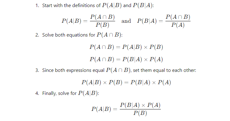
And there you have it—that’s Bayes’ Theorem derived from the basic principles of conditional probability!
Basic Rules and Formulas
Before we dive deeper, let’s refresh some essential probability rules that we’ll use along the way.
- Product Rule (Multiplication Rule):

This rule helps you find the probability of both events A and B occurring.
2. Total Probability Theorem:
If events B1,B2,…,Bn are mutually exclusive and exhaustive, then for any event A:

- This rule allows you to calculate the total probability of event A based on different scenarios Bi.
Transitional Phrase: “By keeping these rules in mind,” you’ll find it much easier to navigate through probability problems and apply Bayes’ Theorem effectively.
Visualizing with Probability Trees and Venn Diagrams
Sometimes, a picture is worth a thousand words. Visual tools like probability trees and Venn diagrams can make these concepts more intuitive.
Probability Trees
Imagine you’re dealing with a deck of cards, and you want to find the probability of drawing an ace followed by a king without replacement.
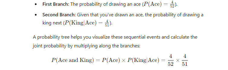
Transitional Phrase: “This might surprise you:” Visualizing with a probability tree makes complex calculations feel much more straightforward.
Venn Diagrams
Venn diagrams are perfect for visualizing how events overlap.
- Circles Represent Events: Each circle represents an event, like A or B.
- Overlap Areas: The intersection where circles overlap represents P(A∩B), the probability of both events occurring.
For example, suppose you’re analyzing customer data:
- Event A: Customers who bought product X.
- Event B: Customers who responded to a marketing email.
The overlap helps you see customers who both bought product X and responded to the email, aiding in calculating conditional probabilities.
Transitional Phrase: “You might be wondering,” how does this help with Bayes’ Theorem? Well, these visuals make the relationships between different probabilities clearer, which is essential when applying Bayes’ Theorem.
Practical Examples
Let’s bring Bayes’ Theorem to life with some practical examples. Trust me, once you see it in action, you’ll appreciate its power even more.
Medical Diagnosis Scenario
Imagine you’re a doctor faced with a challenging situation. A patient comes to you worried that they might have a rare disease. You have a diagnostic test available, but how reliable is it in this context? Let’s dive in and figure it out together.
Problem Statement
Here’s the deal:
- Disease Prevalence: The disease affects 1% of the population.
- Test Accuracy:
- True Positive Rate: If a person has the disease, the test is positive 99% of the time.
- False Positive Rate: If a person doesn’t have the disease, the test is still positive 1% of the time.
You might be thinking, “If the test is 99% accurate, a positive result means the patient almost certainly has the disease, right?” Let’s crunch the numbers and see.
Calculations
Step 1: Define the Probabilities
- P(Disease): Probability that a randomly selected person has the disease = 1% or 0.01.
- P(Positive | Disease): Probability of testing positive if you have the disease = 99% or 0.99.
- P(Positive | No Disease): Probability of testing positive if you don’t have the disease (false positive rate) = 1% or 0.01.
Step 2: Compute P(Disease | Positive) Using Bayes’ Theorem
We want to find P(Disease | Positive): the probability that a person actually has the disease given that they tested positive.
Bayes’ Theorem tells us:

But first, we need to find P(Positive), the overall probability of testing positive.
Compute P(Positive):
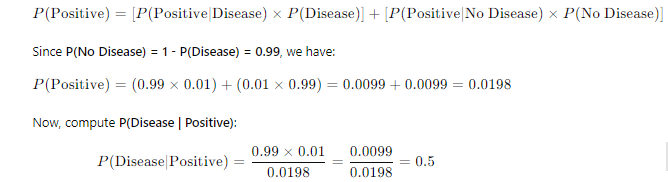
So, even with a positive test result, there’s only a 50% chance that the patient actually has the disease!
Interpretation of Results
This might surprise you: Despite the test being 99% accurate, the probability that the patient has the disease after a positive test is just 50%. Why is that?
Understanding False Positives
Because the disease is rare, the number of false positives can be significant compared to the number of true positives. Out of 10,000 people:
- 100 people have the disease (1% of 10,000).
- 99 of them will test positive (99% of 100).
- 9,900 people do not have the disease.
- 99 of them will also test positive (1% false positive rate).
So, there are 198 positive tests, but only 99 are true positives.
Implications for Medical Decisions
As a healthcare professional, this tells you that a positive test result isn’t definitive. You need to consider additional tests or factors before making a diagnosis. It’s crucial to understand the impact of disease prevalence and test accuracy on interpreting results.
Spam Email Filtering
Ever wondered how your email service sorts out spam from important messages? Bayes’ Theorem is working behind the scenes to keep your inbox clean.
How Spam Filters Use Bayes’ Theorem
Spam filters use Bayesian methods to calculate the probability that an email is spam based on its content. By analyzing word frequencies in spam versus legitimate emails, the filter updates its understanding as more data comes in.
Analyzing Word Frequencies
Let’s say the word “lottery” appears frequently in spam emails but rarely in legitimate ones. The filter considers:
- P(Spam): The overall probability that any email is spam.
- P(“Lottery” | Spam): Probability that the word “lottery” appears in spam emails.
- P(“Lottery” | Not Spam): Probability that the word “lottery” appears in legitimate emails.
Example with Word Probabilities
Suppose:
- P(Spam) = 0.3 (30% of emails are spam).
- P(“Lottery” | Spam) = 0.4
- P(“Lottery” | Not Spam) = 0.01
We want to find P(Spam | “Lottery”): the probability that an email is spam given it contains “lottery”.
First, compute P(“Lottery”):
P(“Lottery”)=[P(“Lottery”∣Spam)×P(Spam)]+[P(“Lottery”∣Not Spam)×P(Not Spam)] P(“Lottery”)=(0.4×0.3)+(0.01×0.7)=0.12+0.007=0.127P
Now, apply Bayes’ Theorem:

So, there’s about a 94.5% chance that an email containing “lottery” is spam.
Calculating the Probability an Email is Spam Given Certain Keywords
By continuously updating these probabilities as more emails are processed, the spam filter becomes more effective over time. It learns from new data, adjusting to spammers’ evolving tactics.
Machine Learning Classification
Now, let’s explore how Bayes’ Theorem is foundational in machine learning, particularly in the Naive Bayes Classifier.
Naive Bayes Classifier Explained
The Naive Bayes Classifier is a simple yet powerful algorithm used for classification tasks. It applies Bayes’ Theorem with the assumption that features are independent given the class label.
You might be thinking, “Features aren’t always independent in real life.” That’s true, but this “naive” assumption simplifies computations and often works surprisingly well.
Assumption of Feature Independence
The classifier assumes that the presence or absence of a particular feature doesn’t affect the presence of any other feature, given the class.
Application in Text Classification
Let’s say you’re building a sentiment analysis model to determine if movie reviews are positive or negative.
- Classes: Positive and Negative sentiment.
- Features: Words used in the review.
Sentiment Analysis Example
Suppose you have the following probabilities based on training data:
- P(Positive) = 0.6
- P(Negative) = 0.4
Word probabilities:
| Word | P(Word | Positive) | P(Word | Negative) | |------------|--------------------|--------------------| | "Amazing" | 0.05 | 0.01 | | "Terrible" | 0.01 | 0.04 | | "Plot" | 0.03 | 0.02 |For a review: “Amazing plot”, compute the probabilities.
Calculate P(Positive | “Amazing plot”):
P(Positive∣Review)∝P(Positive)×P("Amazing"∣Positive)×P("Plot"∣Positive)
𝑃(Positive ∣ Review) ∝ 0.6 × 0.05 × 0.03 = 0.0009
Calculate P(Negative | “Amazing plot”):
P(Negative∣Review)∝0.4×0.01×0.02=0.00008Since 0.0009 > 0.00008, the classifier predicts the review is positive.
Why It Works
Despite the simplification, the Naive Bayes Classifier performs well in practice, especially in text classification tasks where the dimensionality is high, and the independence assumption holds reasonably well.
Applications in Data Science and Machine Learning
Bayes’ Theorem isn’t just a fascinating mathematical concept—it’s a powerful tool that you can apply in various areas of data science and machine learning. Let’s explore how you can harness its potential in real-world scenarios.
Bayesian Inference
Parameter Estimation
Imagine you’re building a model to predict housing prices. You start with some initial guesses about the parameters—these are your prior probabilities. As you collect more data, you update these parameters to better fit the observed data. This process is known as Bayesian inference.
Here’s the deal: Instead of estimating a single value for a parameter, Bayesian inference treats parameters as random variables with probability distributions. This allows you to quantify the uncertainty in your estimates.
Example:
Suppose you’re estimating the average height of adult males in a city. You might start with a prior belief that the average height is around 175 cm with some uncertainty. As you gather height measurements from a sample of the population, you update your belief using Bayes’ Theorem. The result is a posterior distribution that reflects both your prior belief and the new data.
Transitional Phrase: “You might be wondering,” why go through all this trouble? Well, this approach provides a more comprehensive understanding of the parameter estimates, including the confidence you can place in them.
Updating Beliefs with New Data
Sequential Data Analysis
In the fast-paced world of data science, new data streams in constantly. Bayesian methods shine here because they allow you to update your models incrementally.
Example:
Let’s say you’re monitoring the click-through rate (CTR) of an online ad campaign. Initially, you have limited data, but as more users interact with the ad, you can update your estimates of the CTR in real-time.
Transitional Phrase: “Think about it this way:” Each new piece of data is like a puzzle piece that helps you see the bigger picture more clearly. Bayesian updating lets you refine your predictions without starting from scratch each time.
A/B Testing and Decision Making
Choosing Between Competing Hypotheses
A/B testing is a staple in data-driven decision-making. Whether you’re testing website designs or marketing strategies, Bayes’ Theorem can help you determine which option performs better.
Example:
Suppose you’re comparing two versions of a webpage—Version A and Version B. Version A has a conversion rate of 5%, and Version B has 6%. Traditional methods might declare Version B the winner based on this data alone.
Transitional Phrase: “But here’s the kicker:” Bayesian A/B testing allows you to calculate the probability that Version B is better than Version A, given the observed data. This probabilistic approach accounts for uncertainty and can prevent you from making hasty decisions based on limited data.
Comparison with Frequentist Statistics
Advantages and Limitations
You might be asking yourself, “How does Bayesian statistics differ from the traditional frequentist approach?”
Advantages of Bayesian Methods:
- Incorporation of Prior Knowledge: You can include existing knowledge or expert opinions in your analysis.
- Probability Statements About Parameters: Bayesian methods allow you to make direct probability statements about parameters (e.g., “There’s a 95% chance the conversion rate is between X and Y”).
- Flexibility: They are well-suited for complex models and can handle missing data effectively.
Limitations:
- Computational Complexity: Bayesian methods can be computationally intensive, especially with large datasets.
- Choice of Priors: Selecting an appropriate prior can be subjective and may influence results significantly.
Frequentist Methods:
- Objective Approach: They don’t require prior distributions, which eliminates subjectivity but also ignores prior knowledge.
- Simpler Computations: Often less computationally demanding.
Transitional Phrase: “So, what’s the bottom line?” Both approaches have their merits, and the choice between them often depends on the specific problem you’re tackling and your philosophical stance on statistics.
Conclusion
We’ve journeyed through the fascinating landscape of Bayes’ Theorem, exploring its foundational concepts and practical applications. From medical diagnoses and spam filtering to machine learning algorithms and A/B testing, Bayes’ Theorem serves as a versatile tool in your data science toolkit.
Transitional Phrase: “In a world overflowing with data,” the ability to update your beliefs and models as new information emerges is invaluable. Bayes’ Theorem empowers you to make informed decisions under uncertainty, a common scenario in real-world data science projects.
Remember, the essence of Bayesian thinking is adaptability. As you continue your data science endeavors, consider how incorporating Bayesian methods can enhance your analyses and lead to more robust conclusions.