
Imagine this: you’ve built a model that works well for a standard task, say image classification, using common loss functions like Mean Squared Error (MSE) or Binary Cross-Entropy. Everything runs smoothly—until you encounter a unique problem where these built-in losses don’t quite capture the true performance of your model. Perhaps your objective is more nuanced, like optimizing for customer churn, where misclassifying a ‘churn’ is way more costly than a ‘non-churn’. This is where custom loss functions come into play.
You see, built-in loss functions are designed for general-purpose tasks, but they often fall short when you need to incorporate domain-specific knowledge, balance multiple objectives, or handle special cases such as imbalanced datasets. You don’t want to settle for a suboptimal model just because the default tools aren’t cutting it, right? That’s where creating your own loss function empowers you to align the model’s learning process with the actual goals of your project.
When to Use Custom Loss Functions
So, when exactly should you consider writing your own loss function? Let me walk you through a few scenarios:
- Multi-Objective Optimization: Let’s say your model is tackling more than one objective at a time—think of a self-driving car needing to balance speed with safety. A custom loss allows you to weigh each objective based on your priorities.
- Custom Regularization: Sometimes, regularizing your model using standard methods like L2 (Ridge) or L1 (Lasso) isn’t enough. You might need domain-specific constraints—for instance, penalizing model complexity based on specific feature interactions rather than just overall weights.
- Handling Imbalanced Datasets: When the classes in your dataset are imbalanced, a regular cross-entropy loss can be misleading. You’d need a custom solution to ensure your model doesn’t favor the majority class at the expense of minority classes.
What You’ll Learn
Here’s the deal: in this blog, I’m going to show you how to design custom loss functions that solve these complex challenges. We’ll get into hands-on code examples, covering both PyTorch and TensorFlow, so that by the end, you’ll be confident in implementing custom losses that elevate your models to a whole new level. We’ll also cover the nuances of balancing multiple losses, handling non-differentiable objectives, and even debugging common issues when building these functions.
Key Considerations When Designing a Custom Loss Function
Mathematical Formulation
Let’s start with the heart of the matter: the math. You might be wondering, how do you take a specific goal or metric and translate it into a differentiable loss function? It all boils down to ensuring that your loss function captures the essence of the objective you’re trying to optimize, while being compatible with your model’s learning algorithm—typically gradient-based methods.
For example, say you’re optimizing for F1-score rather than accuracy. Directly using F1 as a loss is tricky because it involves precision and recall, which are non-differentiable. So, what do you do? You approximate. You can derive a differentiable surrogate for F1, such as a custom function that mimics the behavior of F1 while still allowing gradients to be calculated. This type of approximation is crucial when the real-world metric you care about doesn’t lend itself to straightforward optimization.
Here’s a practical trick: Always make sure your custom loss is smooth and differentiable, at least in regions where the model needs to learn. Non-smooth functions can lead to erratic gradient updates, resulting in unstable training.
Gradient Computation
This might surprise you, but when you’re writing a custom loss function, you don’t have to worry too much about computing gradients manually. Modern frameworks like TensorFlow and PyTorch have your back here. Thanks to automatic differentiation (autograd in PyTorch, or GradientTape in TensorFlow), you can focus on defining the loss itself, and the framework will handle the heavy lifting of calculating the gradients.
For instance, in PyTorch, all you need to do is subclass nn.Module and implement the forward() method for your custom loss. Autograd will automatically calculate the gradients of your loss function with respect to the model’s parameters during backpropagation. In TensorFlow, the process is similar: you simply define the loss and let tf.GradientTape handle the rest.
Example time: Let’s say you want to implement a custom Mean Absolute Percentage Error (MAPE) loss function in PyTorch:
import torch
import torch.nn as nn

class MAPELoss(nn.Module):
    def forward(self, predicted, target):
        return torch.mean(torch.abs((target - predicted) / target)) * 100
The beauty here is that you don’t need to worry about how gradients are calculated—the framework takes care of it. This frees you up to focus on the creative part: defining losses that match your unique objectives.
Non-differentiable Objectives
Here’s where things get a little tricky. Some objectives aren’t naturally differentiable, but you still need to optimize them. How do you handle that?
Let’s take area under the curve (AUC) as an example. The AUC score is a common evaluation metric in classification tasks, but it’s not directly differentiable. In such cases, you’ll need to rely on surrogate loss functions—these are differentiable approximations that encourage the model to improve performance on the original, non-differentiable metric.
You can also use relaxation techniques to smooth out non-differentiable regions. One popular method is to use the softmax function as a smooth approximation to max functions, which can help when dealing with ranking-based losses.
For instance, let’s say you need to build a custom loss that minimizes the Hinge Loss, used commonly in SVMs for binary classification. While hinge loss is piecewise linear and not differentiable at 0, you can use a smooth approximation like the soft-hinge function:
def soft_hinge_loss(y_true, y_pred, margin=1.0):
    return tf.reduce_mean(tf.maximum(0., margin - y_true * y_pred))
By leveraging these techniques, you can still achieve effective gradient-based optimization, even when dealing with tricky non-differentiable objectives.
Building a Custom Loss Function in PyTorch
Step-by-Step Guide
Now that we understand when and why to create custom loss functions, let’s move on to building one in PyTorch. You’ll see that PyTorch makes this process intuitive, and once you’ve gone through this example, you’ll feel more confident building any custom loss function for your specific needs.
Let’s start with the basics. Every custom loss function in PyTorch is essentially a subclass of nn.Module. Why? Because that’s how PyTorch organizes its layers and operations—loss functions are just another operation applied to your model’s predictions.
Here’s the structure we’ll follow:
- Subclass
nn.Module: This gives you access to PyTorch’s model components, including automatic differentiation. - Define the
forward()method: This is where the real action happens. Theforward()method takes in predictions and targets (the true values) and returns the computed loss.
Now, here’s the deal: you don’t need to manually compute the gradients for your loss function. PyTorch’s torch.autograd handles that for you behind the scenes, using automatic differentiation. This allows PyTorch to compute the gradients of the loss with respect to all the parameters in the model during backpropagation.
Code Example: Custom Mean Squared Logarithmic Error (MSLE) Loss Function
Let’s build a practical example—a Mean Squared Logarithmic Error (MSLE) loss function. You might be wondering why you’d use MSLE instead of regular MSE. Well, MSLE penalizes underestimations more than overestimations, which is useful when you’re dealing with datasets where small values are more significant, or when logarithmic growth is expected in the data.
Here’s the code:
import torch
import torch.nn as nn

class MSLELoss(nn.Module):
    def __init__(self):
        super(MSLELoss, self).__init__()

    def forward(self, predicted, target):
        return torch.mean((torch.log(1 + predicted) - torch.log(1 + target))**2)
Let’s break it down:
__init__()Method: We initialize the custom loss class by calling the parent constructor (super(MSLELoss, self).__init__()). This setup allows us to inherit all the necessary functionality fromnn.Module, including automatic differentiation.forward()Method: This is where the magic happens. The method takes in two arguments—predictedandtarget—and applies the MSLE formula:
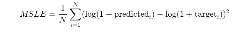
- By using torch.log(1 + predicted) and torch.log(1 + target), we’re ensuring that our loss function works even when the predicted values or targets are small or zero.
Why the extra 1? You might have noticed that we’re adding 1 before taking the log. This ensures that we don’t encounter issues with undefined log(0) when our model predicts or targets zero values. It’s a small tweak that makes a big difference in stability.
Testing the Custom Loss
You might be wondering: How do you use this custom loss in a real model? It’s actually pretty simple. PyTorch treats your custom loss just like any built-in loss function, so you can integrate it into your training loop seamlessly.
Let’s walk through an example using a regression model. Here, we’ll create a dummy dataset, build a simple linear regression model, and use the MSLE loss function to optimize it.
import torch
import torch.optim as optim

# Dummy data (regression problem)
X = torch.randn(100, 1)
y = 3 * X + 1 + 0.1 * torch.randn(100, 1)

# Simple linear regression model
model = torch.nn.Linear(1, 1)

# Custom MSLE loss function
criterion = MSLELoss()

# Optimizer
optimizer = optim.SGD(model.parameters(), lr=0.01)

# Training loop
for epoch in range(100):
    # Forward pass: Compute predicted y by passing X to the model
    y_pred = model(X)

    # Compute the loss using the custom MSLE loss function
    loss = criterion(y_pred, y)

    # Backpropagation and optimization
    optimizer.zero_grad()  # Zero the gradients before running the backward pass
    loss.backward()        # Compute gradients
    optimizer.step()       # Update model parameters

    if epoch % 10 == 0:
        print(f'Epoch [{epoch}/100], Loss: {loss.item():.4f}')
Here’s what’s happening in the code:
- We define a simple linear regression model with one input and one output feature.
- The MSLE loss function we just built is assigned as the criterion for calculating the error between predictions and actual targets.
- We use Stochastic Gradient Descent (SGD) as our optimizer.
- The training loop runs for 100 epochs, where in each epoch, we:
- Pass the input
Xto the model to get predictions. - Calculate the loss using our custom MSLE function.
- Perform backpropagation to compute gradients (
loss.backward()), which PyTorch handles for us using automatic differentiation. - Finally, we update the model parameters using
optimizer.step().
- Pass the input
By printing out the loss every 10 epochs, you’ll see how the model converges over time using your custom loss function.
That’s how simple it is to define and use a custom loss function in PyTorch. The key takeaway is that PyTorch’s automatic differentiation mechanism makes this process smooth and efficient—you focus on designing the loss, and the framework handles the gradient computations. From here, you can start experimenting with more complex, domain-specific losses that give your models a competitive edge.
Building a Custom Loss Function in TensorFlow/Keras
Step-by-Step Guide
When it comes to building custom loss functions in TensorFlow/Keras, the process is very similar to what we’ve already seen with PyTorch—yet with its own nuances. Keras makes custom loss functions straightforward, allowing you to define them as regular Python functions or as Keras layers. What makes TensorFlow especially interesting is the ability to harness tf.GradientTape to manage automatic differentiation.
Here’s the deal: much like PyTorch, TensorFlow handles the gradient calculations automatically during backpropagation, which means you can focus entirely on the logic of the loss function. But, if you need more control—especially when debugging complex models—you can directly use tf.GradientTape to compute gradients, inspect them, and manipulate them as needed.
Defining the Custom Loss Function in TensorFlow/Keras
Let’s talk about the structure. A custom loss function in Keras is simply a Python function that takes the true values (y_true) and the model’s predicted values (y_pred) as inputs. It then returns the computed loss.
Let’s say we want to implement a Custom Huber Loss. You might be thinking, why Huber loss? Well, the Huber loss is great when you want a combination of the robustness of Mean Absolute Error (MAE) and the smoothness of Mean Squared Error (MSE). When the error is small, Huber behaves like MSE, but when the error is large, it switches to MAE, preventing outliers from having too much influence.
Here’s how you can implement it:
import tensorflow as tf

def custom_huber_loss(y_true, y_pred, delta=1.0):
    error = y_true - y_pred
    is_small_error = tf.abs(error) <= delta
    squared_loss = 0.5 * tf.square(error)
    linear_loss = delta * (tf.abs(error) - 0.5 * delta)
    return tf.where(is_small_error, squared_loss, linear_loss)
Breaking It Down:
y_true - y_pred: This is the core of any loss function—the difference between what your model predicts and the actual values.tf.abs(error) <= delta: We use this to identify whether the error is “small” (below a thresholddelta). If it’s small, we calculate a squared loss (like MSE), otherwise we calculate a linear loss (like MAE).tf.where(): This is TensorFlow’s way of conditionally applying different operations. If the error is small, we apply the squared loss, and if it’s large, we apply the linear loss.
Using tf.GradientTape for Automatic Differentiation
You might be wondering: why do we care about tf.GradientTape? Well, there are times when you want to inspect or debug how gradients are flowing through your model, especially if your custom loss function is more complex. tf.GradientTape allows you to compute the gradients of your loss function with respect to any variable, giving you control over the backpropagation process.
Here’s an example:
with tf.GradientTape() as tape:
    y_pred = model(X)  # Forward pass
    loss = custom_huber_loss(y_true, y_pred)  # Compute loss
grads = tape.gradient(loss, model.trainable_weights)  # Compute gradients
optimizer.apply_gradients(zip(grads, model.trainable_weights))  # Apply gradients
This snippet shows how to manually compute and apply gradients, but don’t worry—Keras automatically handles this when you compile the model. However, this can be useful for debugging custom loss functions or creating highly customized training loops.
Testing the Custom Loss
Now, let’s see how to integrate this custom loss into a Keras model. You simply define your loss function and use it while compiling the model. The beauty of Keras is how seamlessly it allows you to plug in custom components.
# Build a simple model
model = tf.keras.Sequential([
    tf.keras.layers.Dense(64, activation='relu'),
    tf.keras.layers.Dense(1)
])

# Compile the model with the custom Huber loss
model.compile(optimizer='adam', loss=custom_huber_loss)

# Dummy data
X = tf.random.normal((100, 10))
y = 3 * tf.reduce_sum(X, axis=1, keepdims=True) + 2

# Train the model
model.fit(X, y, epochs=10)
In this example:
- We define a simple Sequential model with two layers.
- We compile the model using the custom Huber loss instead of the standard loss functions like MSE or MAE.
- Finally, we train the model on some dummy data.
This process is no different than using any built-in loss function, which makes TensorFlow/Keras extremely user-friendly.
Advanced Custom Loss: Multi-Objective Loss Function
When to Use Multi-Objective Losses
Here’s where things get even more interesting. In many real-world problems, you’ll face scenarios where you need to optimize for more than one objective at the same time. Let me give you an example:
Suppose you’re working on an image segmentation task. You don’t just care about correctly classifying each pixel (accuracy), but you also want the boundaries between objects to be sharp and well-defined (localization). In this case, you’d combine two losses—one for classification and one for localization.
Here’s another example: Imagine you’re building a fraud detection model, where you need to balance accuracy with fairness. You can’t have your model unfairly penalizing certain groups, so you’d combine a loss function for prediction accuracy with a fairness constraint.
Code Example: Weighted Combination of Losses
So, how do you create a multi-objective loss function? It’s as simple as weighting and combining individual loss functions. In PyTorch, for example, you can create a custom class to combine multiple losses:
import torch.nn as nn

class CustomMultiLoss(nn.Module):
    def __init__(self, weight_1=0.5, weight_2=0.5):
        super(CustomMultiLoss, self).__init__()
        self.weight_1 = weight_1
        self.weight_2 = weight_2
        self.loss_1 = nn.MSELoss()
        self.loss_2 = nn.L1Loss()

    def forward(self, predicted, target):
        return self.weight_1 * self.loss_1(predicted, target) + \
               self.weight_2 * self.loss_2(predicted, target)
In this example:
weight_1andweight_2represent the importance you assign to each loss. You can tune these weights depending on the relative importance of each objective.loss_1is Mean Squared Error (MSE) andloss_2is Mean Absolute Error (MAE). These two losses capture different aspects of error, and combining them gives you more control over the model’s learning process.
Explaining the Logic
Why use a weighted average? It gives you the flexibility to prioritize one objective over another. For example, if you’re optimizing for both accuracy and fairness, but you care more about accuracy, you would assign a higher weight to the accuracy loss and a lower weight to the fairness loss.
This might surprise you, but multi-objective optimization isn’t just about arbitrarily assigning weights. There’s a whole field called Pareto Optimality, where instead of using fixed weights, you let the model explore trade-offs between objectives dynamically during training. This can be especially powerful when dealing with competing objectives like speed vs. accuracy.
Real-World Example: Multi-Objective Loss in Image Segmentation
Let’s take a practical example from image segmentation—a task where you want to classify pixels while also ensuring that the boundaries between objects are precise. In this case, you might combine a cross-entropy loss (for pixel classification) with a Dice loss (for segmentation boundary accuracy).
def combined_loss(y_true, y_pred):
    cross_entropy = tf.keras.losses.BinaryCrossentropy()(y_true, y_pred)
    dice_loss = 1 - tf.reduce_mean((2 * tf.reduce_sum(y_true * y_pred) + 1) /
                                   (tf.reduce_sum(y_true) + tf.reduce_sum(y_pred) + 1))
    return 0.5 * cross_entropy + 0.5 * dice_loss
This example combines:
- Binary Cross-Entropy: to ensure each pixel is correctly classified.
- Dice Loss: to improve the segmentation boundary by maximizing the overlap between predicted and true masks.
Custom Loss for Imbalanced Data
Addressing Class Imbalance
You might be wondering: why don’t standard loss functions like binary cross-entropy work well for imbalanced datasets? Here’s the deal: in an imbalanced dataset, one class (usually the negative class) vastly outnumbers the other (positive class). When you use regular cross-entropy loss in such cases, the model can get away with simply predicting the majority class most of the time. In fact, it can still achieve high accuracy, but at the expense of recall and precision for the minority class—leading to poor performance for the class you care most about.
This is a classic case where you need to modify your loss function to penalize misclassifications on the minority class more heavily than those on the majority class. One of the most effective ways to address this is by introducing class weights to your binary cross-entropy loss.
Weighted Cross-Entropy Loss
Let me show you a simple way to extend the standard binary cross-entropy to handle imbalanced classes. By weighting the loss function, you’re telling the model to focus more on the minority class, ensuring that those predictions contribute more to the loss function.
Here’s a detailed code example:
import tensorflow as tf

def weighted_binary_crossentropy(y_true, y_pred, weight):
    bce = tf.keras.losses.BinaryCrossentropy()
    # Create a weight vector that assigns more weight to the minority class
    weight_vec = y_true * weight + (1 - y_true)
    return bce(y_true, y_pred) * weight_vec
Breaking It Down:
weight: This is the class weight you manually set to give more importance to the minority class. For instance, if the positive class is rare, you’d assign a higher weight to it (say, 10:1 or 100:1, depending on the imbalance ratio).weight_vec: This vector adjusts the standard binary cross-entropy loss for each class. If the target class is1, it multiplies the loss by the specifiedweight; otherwise, the loss remains unchanged.
Why this works: By applying higher penalties to errors made on the minority class, the model is encouraged to “pay more attention” to it during training. This helps improve performance metrics like recall, precision, and F1-score—key metrics in imbalanced classification tasks like fraud detection or medical diagnosis.
Testing the Weighted Loss Function
You’d integrate this into your Keras model just like any other loss function. For example:
# Compile your Keras model with the custom weighted loss function
model.compile(optimizer='adam',
              loss=lambda y_true, y_pred: weighted_binary_crossentropy(y_true, y_pred, weight=10))
This method is especially powerful for handling cases where misclassifications of the minority class have serious real-world consequences, such as detecting anomalies or rare events.
Regularization-Based Custom Losses
Adding Custom Regularizers
Now let’s talk about regularization. Regularization isn’t just about controlling overfitting—it’s also a tool you can customize to reflect domain-specific constraints. You might already be familiar with standard L1 (Lasso) and L2 (Ridge) regularization, but custom regularizers allow you to apply penalties that suit your model’s specific needs.
For example, you might want to penalize specific parameters, enforce sparsity, or even design a custom regularizer that reflects business rules or domain-specific knowledge. The beauty of Keras is that it makes adding these regularizers to your loss function incredibly easy.
Example: Custom L1-L2 Regularization
Here’s a practical example where you combine L1 and L2 regularization into a custom loss function. This gives you control over both the sparsity (L1) and the smoothness (L2) of the model’s weights.
import tensorflow as tf

def custom_loss_with_regularization(y_true, y_pred, model, l1=0.01, l2=0.01):
    # Calculate the standard loss (e.g., MSE)
    loss = tf.keras.losses.mean_squared_error(y_true, y_pred)

    # Add L1-L2 regularization based on model parameters (weights)
    regularizer = tf.add_n([tf.keras.regularizers.l1_l2(l1, l2)(w) for w in model.trainable_weights])

    # Return the combined loss (regular loss + regularization penalty)
    return loss + regularizer
What’s Happening Here:
mean_squared_error: We’re calculating the regular MSE loss between the predicted values (y_pred) and the true values (y_true).- L1-L2 Regularizer: We apply a combined L1-L2 regularization to each weight in the model. The
tf.keras.regularizers.l1_l2()function handles the math, penalizing large weights (L2) and enforcing sparsity by shrinking some weights toward zero (L1). - Summing Losses: The final loss is a combination of the MSE loss and the regularization penalty, allowing you to control overfitting and enforce domain-specific constraints simultaneously.
Why Regularization Helps
Here’s why custom regularization matters: In many real-world applications, large weight values can make your model less interpretable and more prone to overfitting. By applying L1 or L2 regularization, you can enforce constraints like sparsity (L1) or prevent individual features from having too much influence on the model (L2). This is especially useful in fields like finance, where interpretability is crucial, or when you’re dealing with high-dimensional data that requires feature selection.
Testing the Regularized Loss
To integrate this custom loss function with regularization into your Keras model, you’d use it like this:
# Assume `model` is your pre-defined Keras model
model.compile(optimizer='adam',
              loss=lambda y_true, y_pred: custom_loss_with_regularization(y_true, y_pred, model))
Now your model will not only minimize the prediction error but will also penalize large or unnecessary weights, improving generalization.
Key Takeaways
In this section, we’ve tackled two advanced but highly practical topics: handling imbalanced data with weighted cross-entropy and incorporating domain-specific constraints using regularization. By customizing your loss function to fit the specific characteristics of your problem, you can ensure that your model focuses on the right objectives and stays generalizable.
These techniques, while often overlooked, can make the difference between a good model and a great one—especially when dealing with real-world challenges like imbalanced datasets or the need for model interpretability.
Debugging and Validating Custom Loss Functions
Common Pitfalls
Here’s the deal: building custom loss functions can be tricky. It’s easy to get lost in the math and logic, but one thing that often comes back to bite you is gradient behavior. You might be running your model and seeing unexpected results like exploding or vanishing gradients. This happens when gradients are either too large or too small during backpropagation, leading to unstable or stalled training.
Exploding gradients usually occur when the loss function amplifies errors too much, especially in deep networks. Your model’s weights can spiral out of control, and the loss becomes NaN. On the flip side, vanishing gradients can make it impossible for your model to learn because the gradients become too small for meaningful updates, especially in complex loss functions with multiple non-linearities.
Another common pitfall? Non-differentiable parts of your custom loss function. If you’ve got sharp edges or discontinuities in your loss function, backpropagation will struggle, leading to poor gradient flow.
Techniques for Debugging
So how do you ensure your custom loss function is behaving as expected? One tried-and-true method is gradient checking. This involves comparing the numerically computed gradient (via finite differences) with the gradients computed by your deep learning framework’s automatic differentiation engine. While you typically don’t need to compute gradients manually, gradient checking is a good sanity check when your custom loss function behaves unexpectedly.
Here’s a simple technique using PyTorch for gradient visualization:
import torch

# Example model, loss, and data
model = torch.nn.Linear(10, 1)
inputs = torch.randn(5, 10)
targets = torch.randn(5, 1)

# Define a simple custom loss function
def custom_loss(y_pred, y_true):
    return torch.mean((y_pred - y_true)**2)

# Forward pass
outputs = model(inputs)
loss = custom_loss(outputs, targets)

# Backward pass
loss.backward()

# Visualize the gradients
for name, param in model.named_parameters():
    if param.requires_grad:
        print(f"Gradient for {name}: {param.grad}")
You might be wondering: Why visualize gradients? Because seeing how gradients propagate through your model can highlight issues like vanishing or exploding gradients. If you notice that the gradients are either too small (close to zero) or too large, you know there’s an issue with either your loss function or the model’s architecture.
Validation on Toy Problems
Before deploying a custom loss function in a real-world scenario, you want to test it on controlled, toy problems. Think of this like debugging code with unit tests. You create small datasets where the expected behavior of your loss function is clear, and then you can validate whether the loss function is working as expected.
Here’s an example. Let’s say you’ve written a custom loss function to predict values close to zero. You’d create a simple linear regression problem where the ground truth values are small. If your loss converges to zero on this toy problem, you’re in good shape.
# Simple toy problem setup for validating a custom loss
X = torch.randn(100, 1)
y = 0.5 * X  # Ground truth: small values

model = torch.nn.Linear(1, 1)
criterion = custom_loss

# Train on the toy problem
optimizer = torch.optim.SGD(model.parameters(), lr=0.01)
for epoch in range(100):
    optimizer.zero_grad()
    outputs = model(X)
    loss = criterion(outputs, y)
    loss.backward()
    optimizer.step()

    if epoch % 10 == 0:
        print(f"Epoch [{epoch}/100], Loss: {loss.item()}")
This validation on toy data ensures that your custom loss function works in simplified conditions before you move on to more complex datasets and architectures.
Optimizing and Tuning Custom Loss Functions
Hyperparameter Tuning
Now, you’ve built your custom loss function, and it seems to be working well. But here’s the kicker: you can always squeeze out more performance by tuning the hyperparameters of your loss function. For instance, when you’re working with multi-objective losses, the weights you assign to each objective can make or break your model’s performance.
Let’s take a real-world example. Suppose you’re training a model for object detection, where the loss is a combination of classification loss and localization loss. The relative importance of these two objectives can be controlled by adjusting their weights in the loss function.
You might be wondering: how do I choose these weights? The answer lies in hyperparameter optimization. You can use techniques like grid search or more sophisticated methods like Bayesian optimization to find the optimal values.
Here’s how you could apply grid search for tuning loss weights in Keras:
from sklearn.model_selection import ParameterGrid
import tensorflow as tf

# Define a function for your custom loss with variable weights
def custom_multi_loss(y_true, y_pred, weight_1, weight_2):
    loss_1 = tf.keras.losses.BinaryCrossentropy()(y_true, y_pred)
    loss_2 = tf.keras.losses.MeanSquaredError()(y_true, y_pred)
    return weight_1 * loss_1 + weight_2 * loss_2

# Example grid of weights to search over
param_grid = {'weight_1': [0.1, 0.5, 1.0], 'weight_2': [0.1, 0.5, 1.0]}

# Create your model
model = tf.keras.Sequential([tf.keras.layers.Dense(1, activation='sigmoid')])

# Grid search
for params in ParameterGrid(param_grid):
    # Compile the model with the current set of weights
    model.compile(optimizer='adam',
                  loss=lambda y_true, y_pred: custom_multi_loss(y_true, y_pred, params['weight_1'], params['weight_2']))

    # Fit the model on your data
    model.fit(X_train, y_train, epochs=10)

    # Evaluate performance
    score = model.evaluate(X_val, y_val)
    print(f"Weights: {params}, Validation Loss: {score}")
In this example, we’re systematically trying different combinations of weights for the multi-objective loss function. You’ll notice that some weight combinations lead to better performance, depending on the dataset and objectives.
Real-World Example
Consider a fraud detection model where you need to tune the balance between precision and recall. You can use Bayesian optimization to find the optimal weight for the recall term in your custom loss function. Libraries like Optuna or Scikit-Optimize can help automate this process, saving you time and effort by focusing the search on the most promising areas of the hyperparameter space.
Conclusion
Key Takeaways
Custom loss functions are a powerful tool that gives you the flexibility to tailor your model’s learning process to the specific needs of your domain. Whether you’re dealing with imbalanced data, multiple objectives, or the need for custom regularization, writing your own loss functions allows you to align the model’s optimization process with the real-world goals you care about.
Remember, though, that designing custom losses comes with challenges like vanishing/exploding gradients, non-differentiable parts, or incorrect gradient flows. Proper debugging with gradient visualization and validation on toy problems will save you from many headaches.
Next Steps
Where do you go from here? Experimentation is key. Try building custom loss functions for complex tasks like reinforcement learning, where reward shaping can benefit from custom losses, or explore unsupervised learning where loss functions might need to encode complex latent relationships. The flexibility you’ve unlocked by mastering custom losses opens doors to pushing the boundaries of what your models can achieve.