
Imagine looking at a photo—what’s the first thing your brain does? It recognizes objects, colors, and even the depth of the scene. This is how our brains process visual representations, and in many ways, computer vision tries to mimic this ability. But here’s the catch: computers need a lot of help to “see” the world the way we do. That’s where visual representations come into play, especially in tasks like image classification, object detection, and segmentation.
You might be wondering: what exactly do we mean by “visual representations”? In computer vision, visual representations are the way we encode an image into a form that a machine can understand. For example, in an image classification task, the computer has to break down an image into numerical features that represent the objects, textures, and patterns within it. It’s the backbone of how systems like facial recognition and autonomous vehicles work.
But here’s the deal: supervised learning, which has been the dominant method for teaching machines to recognize these visual features, depends heavily on labeled data. For every image, you need a human to say, “This is a cat,” or “This is a car.” As you can imagine, this process is expensive and doesn’t scale easily. What if I told you there’s a way to cut down on the need for labeled data? This is where self-supervised learning steps in, and it’s changing the game for visual representations.
What is Contrastive Learning?
At the heart of self-supervised learning is contrastive learning. Now, let’s get into it—because this is where things get exciting. The main idea behind contrastive learning is actually quite intuitive: pull similar things closer together and push different things apart.
Let me give you an example. Imagine you have two photos of a cat. Even if one is taken from a different angle or in different lighting, they still represent the same object. In contrastive learning, these two images are treated as positive pairs, and the model learns to pull their representations closer together. On the other hand, if you throw in a picture of a dog, the model will treat this as a negative pair and push its representation away from the cat images.
Now, to make this work mathematically, we use something called contrastive loss—specifically, InfoNCE loss is often used in this context. The goal of this loss function is to maximize the similarity between positive pairs while minimizing the similarity between negative pairs. Think of it as a system of rewards: the model gets rewarded when it brings similar images together and penalized when it confuses different ones.
Mathematical Definition
Let’s dive into a bit of math, but don’t worry—I’ll keep it straightforward. The contrastive loss is often defined as:

Where:
- sim stands for a similarity metric like cosine similarity or Euclidean distance.
- τ is a temperature parameter that controls how strictly the model pushes apart dissimilar images.
- xi and xjj are positive pairs (for example, two different views of the same image), while xk represents negative samples.
This might look a little daunting, but it’s essentially a way to ensure that positive pairs (similar images) are pushed together in a high-dimensional feature space, and negative pairs are pushed apart. The beauty of this approach is its simplicity and power—you don’t need labeled data to make it work!
Historical Context
Contrastive learning isn’t brand new—it’s actually had quite a journey. You may have come across it in natural language processing (NLP) with models like Word2Vec, where similar words were brought closer together in a high-dimensional space. But its real breakout moment came in computer vision when researchers started applying it to unsupervised visual representation learning. Models like SimCLR and MoCo revolutionized the way we think about visual tasks, allowing machines to learn features from raw, unlabeled images.
And now, here we are—contrastive learning has made its way into all kinds of visual tasks, from image classification to more complex ones like segmentation and detection. The results are nothing short of impressive: models trained with contrastive learning are not only more robust, but they also generalize better to new tasks.
Why Contrastive Learning for Visual Representations?
If you’ve ever worked with computer vision projects, you probably know this frustration: getting labeled data is hard, expensive, and slow. Think about it. For every dataset, you need humans to painstakingly label thousands—sometimes millions—of images. Imagine someone manually labeling whether each image in a dataset contains a cat, dog, tree, or car. Not only is it tedious, but it’s also prone to errors.
The Challenge of Labeled Data
In visual tasks like image classification or object detection, this dependence on labeled data becomes a bottleneck. Here’s the deal: as the complexity of tasks increases, the amount of labeled data you need grows exponentially. Whether it’s training a model to recognize a specific breed of dog or identifying anomalies in medical images, the problem is the same: labeled data is a resource that’s costly to scale.
Self-Supervised Learning Approach
So, what’s the alternative? This is where self-supervised learning—and more specifically, contrastive learning—enters the scene and shakes things up. Rather than relying on humans to tell a model what’s in every image, self-supervised learning lets the model learn from unlabeled data. It’s like teaching a child to recognize objects by giving them clues about what’s similar and what’s different, without spelling everything out.
Contrastive learning plays a key role here by allowing machines to extract useful features from images without needing labeled examples. Instead of telling the model, “This is a cat,” and “This is a dog,” you train the model to understand the relationship between different images: which ones should be close together (positive pairs) and which ones should be far apart (negative pairs). The model learns to build a robust visual understanding based on these relationships alone.
Robustness and Generalization
And here’s the kicker: models trained with contrastive learning tend to be far more robust and generalizable than their supervised counterparts. Why? Because they don’t rely on specific labels—they’re learning the essence of the data itself. Think of it as teaching someone the principles of a language instead of just memorizing a dictionary. These models are better equipped to handle diverse visual tasks, even if the exact data distribution is different from the one they were trained on.
What does this mean for you? It means you can train a model on a massive, unlabeled dataset (which is relatively easy to gather), and that model will be strong enough to transfer to downstream tasks like image segmentation, object detection, or even fine-grained image classification.
Core Methodologies in Contrastive Learning for Visual Representations
Now that you have a good sense of why contrastive learning is so powerful, let’s dig into the how. Contrastive learning typically operates by using self-supervised pretext tasks—tasks where the goal is not to solve a real-world problem directly, but rather to learn useful representations from the data that can later be applied to various downstream tasks. Here’s how it works:
Contrastive Pretext Tasks
One of the clever tricks used in contrastive learning is applying data augmentations to create positive and negative pairs. Think of this as giving the model different “views” of the same image. For example, you might take an image of a cat and generate several augmented versions by cropping, rotating, or changing the brightness. Each of these augmented images becomes part of a positive pair, while images of entirely different objects (like dogs or cars) serve as negative pairs.
What you’re doing is teaching the model to recognize, “Hey, these different views are actually of the same thing,” while simultaneously learning to distinguish between completely different objects. This is what makes contrastive learning so good at building rich, generalizable feature representations—you don’t need explicit labels for this kind of learning to occur.
Popular Models in Contrastive Learning
Let’s talk about the key players in the field of contrastive learning. There have been several standout models that have pushed the boundaries of what’s possible. Here are the big names you should know:
SimCLR
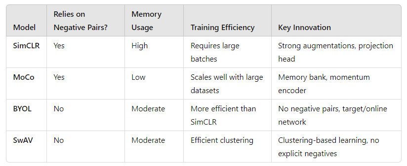
First up is SimCLR (Simple Framework for Contrastive Learning of Visual Representations). SimCLR is known for its simplicity and effectiveness. The key innovation in SimCLR lies in its use of strong augmentations and a projection head—a small neural network added after the backbone that maps the features into a latent space where contrastive learning happens.
In SimCLR, you take two random augmentations of the same image to create positive pairs and other images in the batch serve as negative pairs. The model tries to minimize the distance between the positive pairs while maximizing the distance from negative pairs in this projected space.
MoCo
Next, we have MoCo (Momentum Contrast), which brings in a new twist: the memory bank. MoCo is designed to scale better with large datasets by using a memory bank to store representations from previous batches. What makes MoCo stand out is its ability to maintain consistent feature representations using a momentum encoder, which slowly updates based on past mini-batches.
You might think of MoCo as more efficient for larger datasets, as it doesn’t need a huge batch size like SimCLR. It’s like having a long-term memory of past samples, allowing the model to compare current representations to previously seen images.
BYOL
Here’s where things get really interesting: BYOL (Bootstrap Your Own Latent). Unlike SimCLR and MoCo, BYOL removes the need for negative pairs altogether. That’s right—BYOL learns without explicitly contrasting positive and negative samples. Instead, it focuses entirely on pulling different views of the same image together.
BYOL works by using two neural networks: a target network and an online network. The target network is a slowly evolving version of the online network, and they work together in tandem to learn meaningful representations. Despite the absence of negative pairs, BYOL achieves impressive results in practice.
SwAV
Last but not least is SwAV (Swapping Assignments between Views). SwAV introduces a clustering-based approach to contrastive learning. Instead of just comparing augmented views of the same image, SwAV groups similar features together using unsupervised clustering, creating a sort of “soft” comparison between views.
This allows the model to learn even more fine-grained features, making it particularly effective for complex visual tasks. The clustering mechanism helps group similar images together even without explicit labels, improving the model’s ability to generalize to new data.
Comparison of Approaches
Here’s a quick breakdown to help you compare these methods:
Key Concepts in Contrastive Learning for Visual Tasks
Augmentation Strategies
Imagine taking the same photo from different angles or with various filters—it’s still the same object, right? Well, in contrastive learning, we rely heavily on these kinds of augmentations to create diverse “views” of the same image. The goal is to give the model different perspectives of the same image and teach it to recognize that these different views belong to the same object.
Here’s where things get creative: we use strategies like cropping, color distortion, flipping, and even blurring to create meaningful variations. Think of these augmentations as controlled experiments that force the model to learn more general, robust features. So, even when the image looks slightly different due to cropping or color changes, the model learns that it’s still looking at the same object.
For example, if you have an image of a cat, you could crop the cat’s face or change the lighting, and these become your positive pairs—different views of the same image. The model then learns to bring these pairs closer together in the feature space.
Instance Discrimination
Here’s the deal: in contrastive learning, we treat every single image as its own class. This might sound odd, but it’s called instance discrimination, and it’s a key part of how contrastive learning works. Each image gets its own unique identity, and the model’s job is to distinguish it from all the others, even if they are similar.
Think of it like this: imagine a party where everyone is dressed in similar outfits. Your task is to pick out your friend from the crowd, not by their clothes, but by their distinct characteristics—maybe their height, posture, or the way they walk. In contrastive learning, the model tries to identify each image based on these unique “features,” and it learns to pull different instances apart while grouping different views of the same instance closer together.
Batching and Memory Bank
Now, you might be wondering: how does the model know what’s similar and what’s different, especially with so many images to compare? This is where large batch sizes or memory banks come in.
Contrastive learning works best when it can compare many images at once, which is why large batches are crucial. In models like SimCLR, a bigger batch size means the model has more negative samples to learn from, making the learning process more effective. However, training with large batch sizes requires a lot of computational power, and that’s not always practical.
Here’s the alternative: a memory bank, as used in models like MoCo. Instead of needing a massive batch, the memory bank stores representations of previous batches, allowing the model to use these stored examples as negative pairs. This makes the process more efficient and less reliant on giant batches, making it easier to scale contrastive learning to larger datasets.
The Role of Architectures in Contrastive Learning
Backbone Networks
You’ve probably heard of ResNet, right? It’s one of the most popular backbone architectures used in contrastive learning. But what is a backbone network, and why does it matter?
A backbone network is essentially the feature extractor—the part of the model responsible for taking in raw images and transforming them into useful feature representations. Models like ResNet are commonly used because they’ve been shown to be incredibly effective at extracting high-level features from images, making them a natural fit for contrastive learning tasks.
But here’s the thing: your choice of backbone can have a significant impact on the performance of your contrastive model. The deeper and more powerful the backbone (e.g., ResNet50 vs. ResNet101), the more detailed the representations it can learn. However, deeper networks also come with trade-offs in terms of computational cost and training time, so there’s always a balance to strike.
Projection Heads
Now, let’s talk about something that often gets overlooked but is just as critical: the projection head. After the backbone network extracts features from the image, those features are passed through a projection head, which is typically a small multi-layer neural network.
But why bother with this extra step? The reason is simple: dimensionality reduction. The projection head takes the high-dimensional features learned by the backbone and maps them into a lower-dimensional space where contrastive learning happens. This space is where the model compares positive pairs and pulls them closer while pushing negative pairs apart.
The projection head helps improve the quality of the learned representations, making them more suitable for the contrastive task. Interestingly, in many cases, the features learned by the backbone before the projection head are more useful for downstream tasks (like classification), which is why some models discard the projection head after training is complete.
Metrics and Evaluation of Contrastive Learning Models
Linear Evaluation Protocol
When it comes to evaluating contrastive learning models, one of the most widely used approaches is the linear evaluation protocol. This is where things get interesting because, after all the effort of training a contrastive model, you don’t immediately test it on the actual task. Instead, you freeze the learned representations and then train a simple linear classifier on top of them.
Here’s why this is important: the performance of the linear classifier tells you how well the contrastive model has learned general features. If the classifier performs well, it means the representations are rich and informative. On the other hand, if the performance is poor, it suggests that the learned features aren’t as useful as you’d hoped.
Transfer Learning
You might be wondering: what happens to these learned representations after training? Can you use them for other tasks? Absolutely. In fact, one of the major benefits of contrastive learning is how well the learned visual representations transfer to other tasks.
For instance, you can fine-tune a contrastive model trained on an unlabeled dataset and apply it to tasks like object detection, image segmentation, or medical imaging. The pre-trained model already knows how to extract meaningful features, so when you adapt it to a specific task, you don’t need as much labeled data.
Top-K Accuracy, mAP, and Other Metrics
Finally, let’s talk numbers. How do we actually measure the performance of contrastive learning models?
- Top-K Accuracy: This is a common metric where the model’s prediction is considered correct if the true label is among the top K predicted labels. It’s particularly useful for tasks with many categories, like image classification.
- Mean Average Precision (mAP): This metric is commonly used for object detection tasks. It evaluates how well the model identifies objects and their locations within an image, taking both precision and recall into account.
By using these metrics, you can get a clearer picture of how well your contrastive learning model performs across various tasks.
Conclusion
By now, you’ve seen the immense value that contrastive learning brings to visual representation tasks. From augmentation strategies and instance discrimination to the role of backbone networks and projection heads, every part of the process contributes to learning more robust, generalizable, and transferable visual features. And while the training process may seem complex, the results speak for themselves—these models are revolutionizing how we approach self-supervised learning in computer vision.